In the last post I wrote about inference, marginalization and such for SPNs. Now let us take a look at parameter learning for SPNs.
Toy example
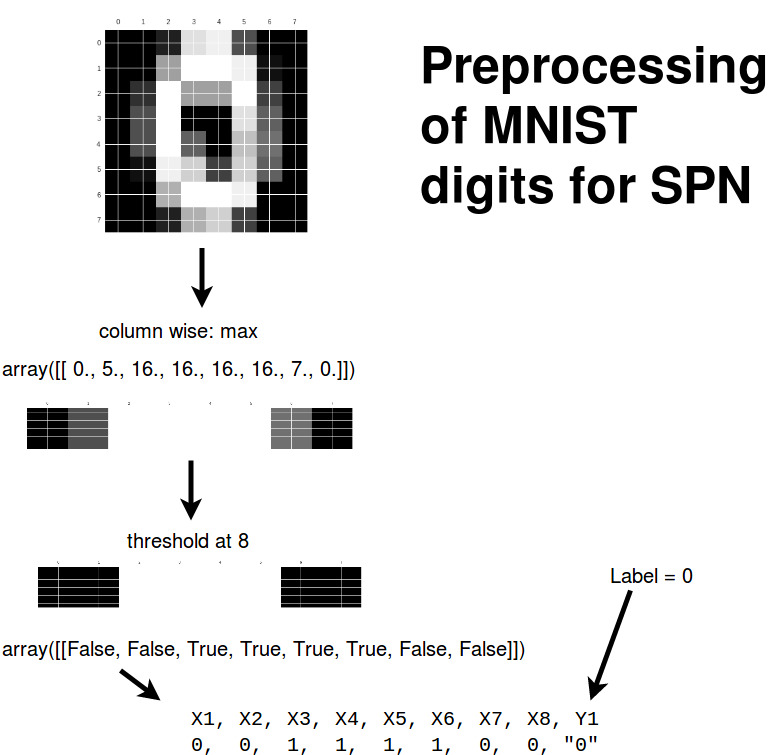
In order to motivate ourselves let’s try to solve a motivating example: We try to estimate the MNIST digits: classifying whether the pixels show a zero or not.
We preprocess the digits as follows to make the SPN small enough for visualization:
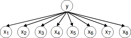
And because we want to do parameter learning we assume that there is already the following Bayes Network given:
Which can be converted into the following SPN:
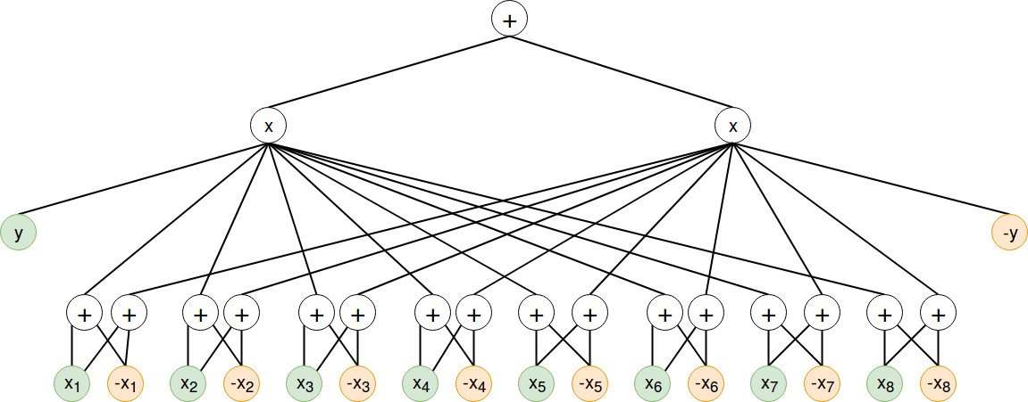
Where we assume the that the weights under the sum nodes are initialized with 0.5.
(The attentive reader might notice that the topology of the SPN makes the usage of SPNs a little bit obsolete. But for the sake of explanation I chose to do it like this.)
Parameter Learning
There are generally two ways to learn the SPN parameters:
- generative learning: modelling P(x) for every y
-
discriminative learning: P(y x)
And there are two methods:
- Expectation Maximization (if we have variables which can’t be observed)
- Gradient Descent
(Note: For deep SPNs there exists a solution to avoid the vanishing gradient called “hard gradient” which maximizes the likelihood of P’(x) instead of P(x). P’(x) is the approximation of the sum of P(x) by its largest term.)
Gradient for discriminative learning
We want to maximize this term: \(\max \nabla log P(y|x)\)
We apply the product rule: \(\max \nabla log {P(y, x) \over P(x)}\)
Which is the same as: \(\ max \nabla log {P(y, x)} - \nabla log { P(x)}\)
P(y, x) is the probability that our network produces the correct output given the input. And P(x) is the total output our network produces.
P(y, x) is just inference and P(x) can be calculated by marginalizing over y.
Illustration
Let’s illustrate all necessary steps to do gradient descent on a SPN.
P(X,Y)
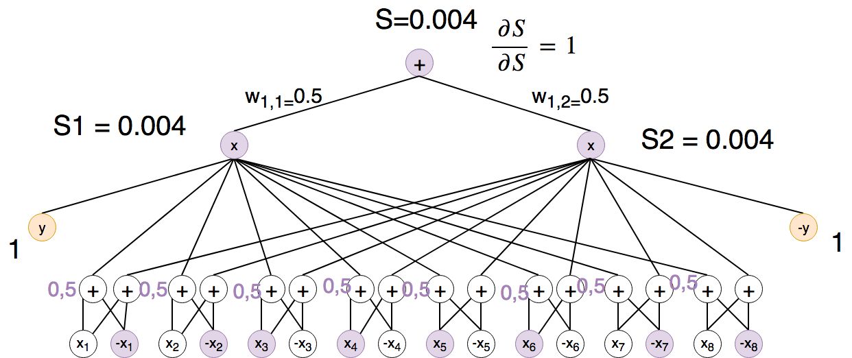
First we calculate P(x,y) by a single forward pass for the training example from the section about preprocessing:
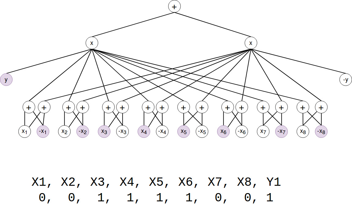
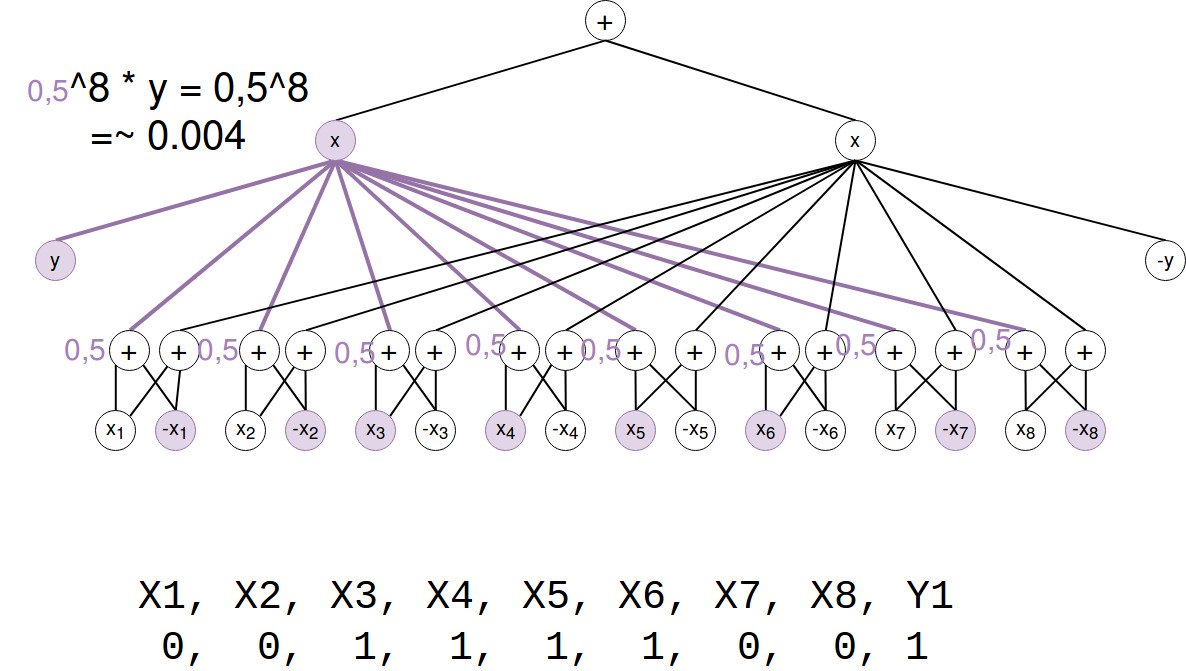
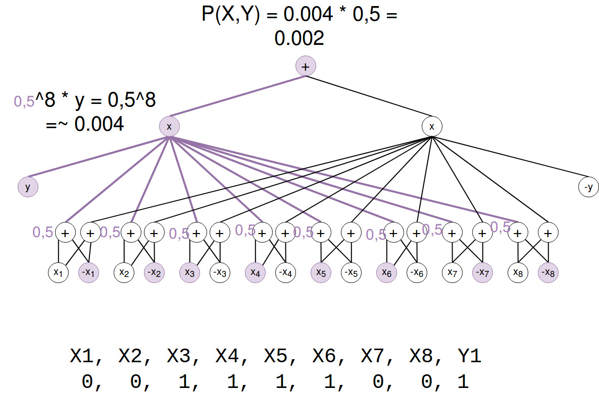
(Note that P(X,Y) = S(x_ind) / Z. Z=1 so we just skipped this.)
Okay, so the probability of our image and the label is 0,4%.
P(X)
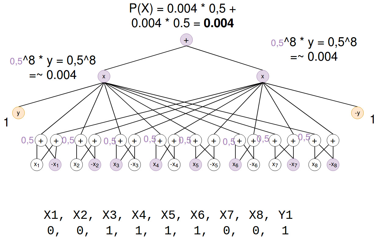
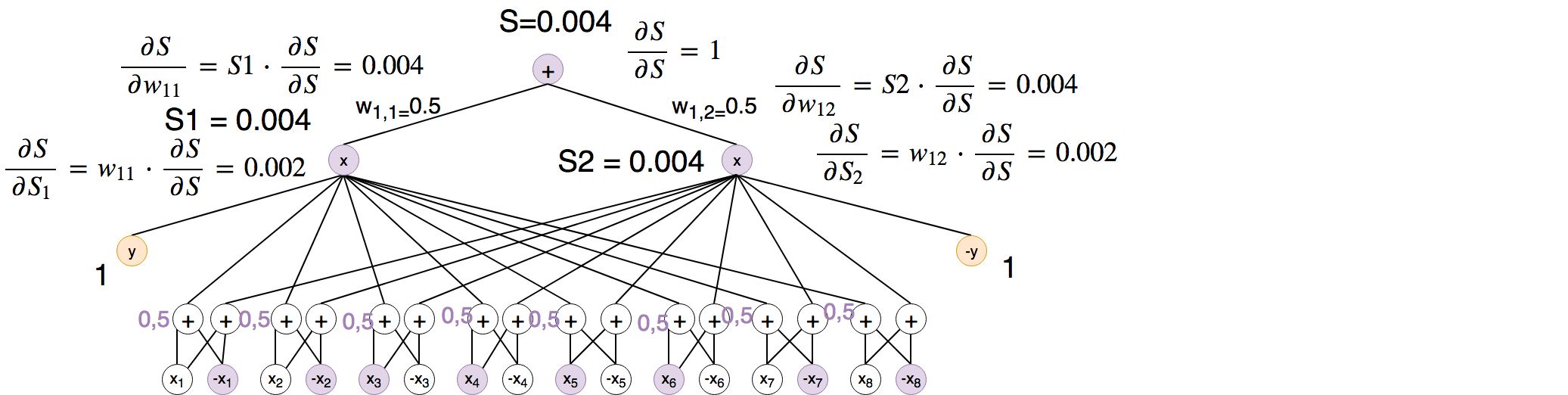
Next step is to marginalize over Y to get P(X):
Backprop
Because we want to maximize the difference between P(Y,X) and P(X) we can say that our error signal is P(Y,X) - P(X) = 0.002. To make this bigger we have to decrease P(X) and increase P(Y,X). But what made P(X) so big? This is what backprop can tell us.
Therefore we are going to backprop the output of P(X) to all its variables:
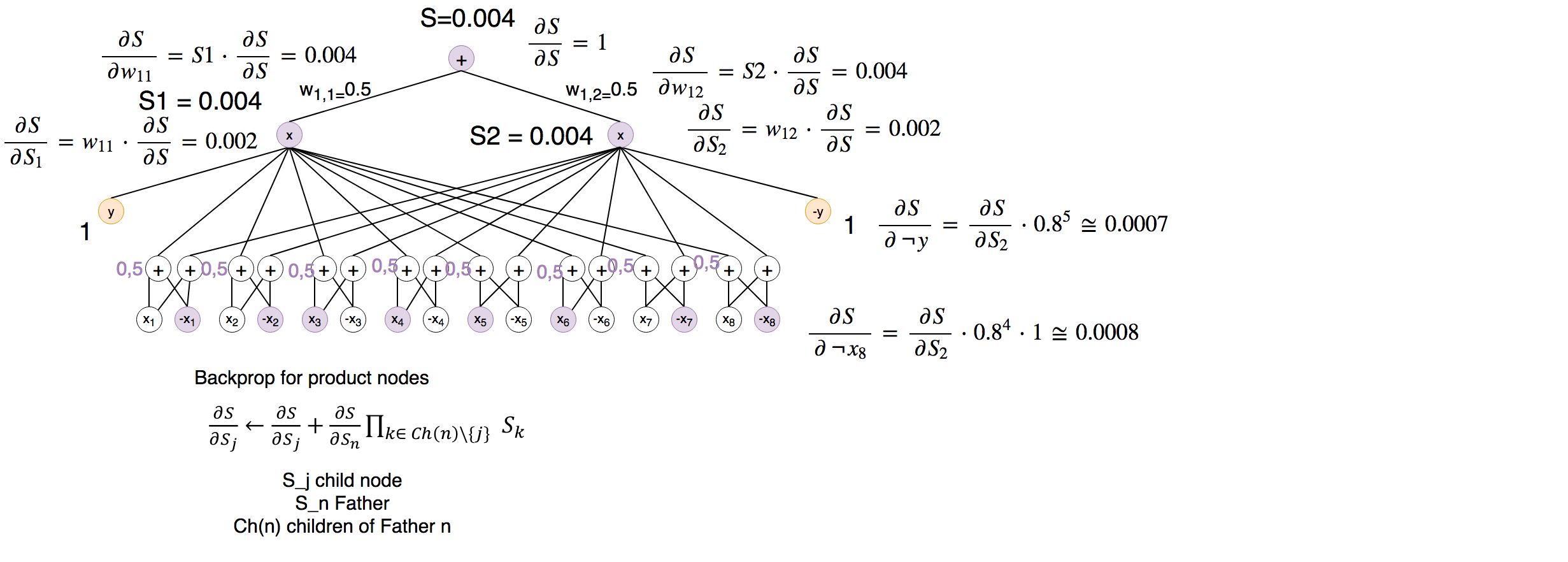
I guess you can imagine how this should work. Luckily there are tools out there which can do this automagically for us ;)
Note: The 0.8^5 should be 0.5^8…
Second part backprop: Now we can calculate the backprop for the P(Y,X)
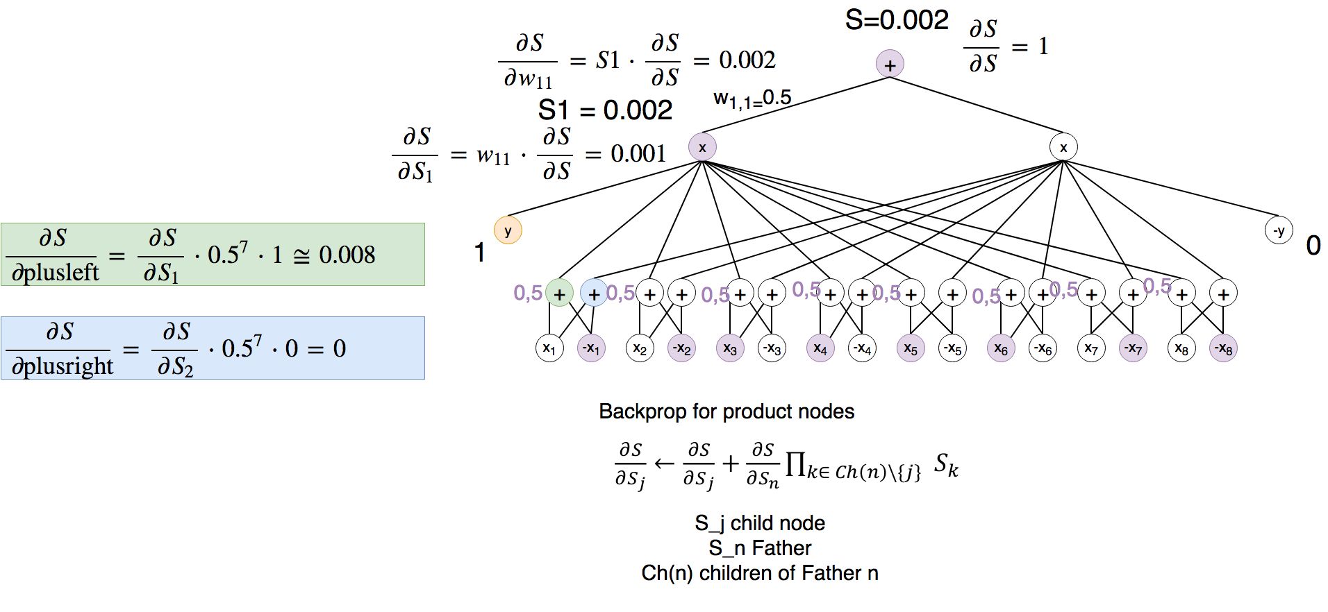
Now we can see that the weights in the lowest layer would be adapted partially to match the inputs. We can already see why the hard gradient could become necessary.
Implementing backprop
It is obviously an easy way to show that this procedure can be used to adapt weights by programming a small example.
Preprocessing
Let’s get the MNIST digits:
import matplotlib.pyplot as plt
import numpy as np

from sklearn.datasets import load_digits

digits = load_digits()

plt.gray()
plt.matshow(digits.images[55])
plt.show()
digits.target[55]
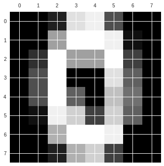
“0”
Now we get the maximum of every column (we did this to keep the SPN reasonably small).
(digits.images.max(axis=1).reshape(-1, 8)>8.0).shape
array([[False, False,  True, ...,  True, False, False],
       [False, False,  True, ...,  True, False, False],
       [False,  True,  True, ...,  True,  True, False],
       ...,
       [False, False,  True, ...,  True, False, False],
       [False, False,  True, ...,  True, False, False],
       [False, False,  True, ...,  True, False, False]])
Preparing tensorflow graph
Please see my post on tensorflow toy examples for the basics: here
import tensorflow as tf

# for working in a notebook
sess = tf.InteractiveSession()

# init weights
weights1 = [0.5, 0.5]
weights2 = [0.5] * 8 * 2 * 2
For every SPN there is a corresponding network polynomial. Which we use to build the computation graph:
# The placeholder for the parameter
x = tf.placeholder(tf.float32)

y = tf.placeholder(tf.float32)

# the weights of the highest layer from left to right
w1 = tf.placeholder(tf.float32)

# the weights of the lowest layer from left to right
w = tf.placeholder(tf.float32)

# the network polynomial which encodes our SPN
f = w1[0] * (
    (x[0]*w[0] + (1-x[0])*w[1]) *
    (x[1]*w[4] + (1-x[1])*w[5]) *
    (x[2]*w[8] + (1-x[2])*w[9]) *
    (x[3]*w[12]+ (1-x[3])*w[13]) *
    (x[4]*w[16]+ (1-x[4])*w[17]) *
    (x[5]*w[20]+ (1-x[5])*w[21]) *
    (x[6]*w[24]+ (1-x[6])*w[25]) *
    (x[7]*w[28]+ (1-x[7])*w[29]) *
    (y)) + \
  w1[1] * (
      (x[0]*w[2]+  (1-x[0]) *w[3]) *
      (x[1]*w[6]+  (1-x[1]) *w[7]) *
      (x[2]*w[10]+ (1-x[2]) *w[11]) *
      (x[3]*w[14]+ (1-x[3]) *w[15]) *
      (x[4]*w[18]+ (1-x[4]) *w[19]) *
      (x[5]*w[22]+ (1-x[5]) *w[23]) *
      (x[6]*w[26]+ (1-x[6]) *w[27]) *
      (x[7]*w[30]+ (1-x[7]) *w[31]) *
      (1-y)
  )

# f(x=0) in interactive session
f.eval(feed_dict={x:data[55], y:digits.target[55]==0, w1:weights1, w:weights2})
The output is: 0.001953125
Which is exactly what we calculated for P(X,Y). :)
We have to manipulate the code a little bit to allow marginalization of P(X):
# The placeholder for the parameter
x = tf.placeholder(tf.float32)

y_true = tf.placeholder(tf.float32)
y_false = tf.placeholder(tf.float32)

# the weights of the highest layer from left to right
w1 = tf.placeholder(tf.float32)

# the weights of the lowest layer from left to right
w = tf.placeholder(tf.float32)

# the network polynomial which encodes our SPN
f = w1[0] * (
    (x[0]*w[0] + (1-x[0])*w[1]) *
    (x[1]*w[4] + (1-x[1])*w[5]) *
    (x[2]*w[8] + (1-x[2])*w[9]) *
    (x[3]*w[12]+ (1-x[3])*w[13]) *
    (x[4]*w[16]+ (1-x[4])*w[17]) *
    (x[5]*w[20]+ (1-x[5])*w[21]) *
    (x[6]*w[24]+ (1-x[6])*w[25]) *
    (x[7]*w[28]+ (1-x[7])*w[29]) *
    (y_true)) + \
  w1[1] * (
      (x[0]*w[2]+  (1-x[0]) *w[3]) *
      (x[1]*w[6]+  (1-x[1]) *w[7]) *
      (x[2]*w[10]+ (1-x[2]) *w[11]) *
      (x[3]*w[14]+ (1-x[3]) *w[15]) *
      (x[4]*w[18]+ (1-x[4]) *w[19]) *
      (x[5]*w[22]+ (1-x[5]) *w[23]) *
      (x[6]*w[26]+ (1-x[6]) *w[27]) *
      (x[7]*w[30]+ (1-x[7]) *w[31]) *
      (y_false)
  )

# f(x=0) in interactive session
f.eval(feed_dict={x:data[55],
                  y_true:1,  # digits.target[55]==0
                  y_false:1,
                  w1:weights1,
                  w:weights2
                 })
Output: 0.00390625 (our 0.004 was approximately correct)
Training
import tensorflow as tf
import random
import matplotlib.pyplot as plt
tf.enable_eager_execution()
# Initialize the weights
weights1 = [0.5, 0.5]
weights2 = [0.5] * 8 * 2 * 2
iterations = 900
break_crit = 0.000001
errors = []
for i in range(iterations):
if i%101==0:
print(i)
with tf.GradientTape(persistent=True) as t:
sample = random.randint(0, 1000)
# The placeholder for the parameter
x = tf.convert_to_tensor(data[sample].astype(np.float32))
t.watch(x)
y_true = (digits.target[sample]==0).astype(np.float32)
y_false = 1-(digits.target[sample]==0).astype(np.float32)
# the weights of the highest layer from left to right
w1 = tf.convert_to_tensor(weights1)
t.watch(w1)
# the weights of the lowest layer from left to right
w = tf.convert_to_tensor(weights2)
t.watch(w)
# P(Y,X)
# the network polynomial which encodes our SPN
s = w1[0] * (
(x[0]*w[0] + (1-x[0])*w[1]) *
(x[1]*w[4] + (1-x[1])*w[5]) *
(x[2]*w[8] + (1-x[2])*w[9]) *
(x[3]*w[12]+ (1-x[3])*w[13]) *
(x[4]*w[16]+ (1-x[4])*w[17]) *
(x[5]*w[20]+ (1-x[5])*w[21]) *
(x[6]*w[24]+ (1-x[6])*w[25]) *
(x[7]*w[28]+ (1-x[7])*w[29]) *
(y_true)) + \
w1[1] * (
(x[0]*w[2]+ (1-x[0]) *w[3]) *
(x[1]*w[6]+ (1-x[1]) *w[7]) *
(x[2]*w[10]+ (1-x[2]) *w[11]) *
(x[3]*w[14]+ (1-x[3]) *w[15]) *
(x[4]*w[18]+ (1-x[4]) *w[19]) *
(x[5]*w[22]+ (1-x[5]) *w[23]) *
(x[6]*w[26]+ (1-x[6]) *w[27]) *
(x[7]*w[30]+ (1-x[7]) *w[31]) *
(y_false)
)
z = w1[0] * (
(1*w[0] + 1*w[1]) *
(1*w[4] + 1*w[5]) *
(1*w[8] + 1*w[9]) *
(1*w[12]+ 1*w[13]) *
(1*w[16]+ 1*w[17]) *
(1*w[20]+ 1*w[21]) *
(1*w[24]+ 1*w[25]) *
(1*w[28]+ 1*w[29]) *
(1)) + \
w1[1] * (
(1*w[2]+ 1 *w[3]) *
(1*w[6]+ 1 *w[7]) *
(1*w[10]+ 1 *w[11]) *
(1*w[14]+ 1 *w[15]) *
(1*w[18]+ 1 *w[19]) *
(1*w[22]+ 1 *w[23]) *
(1*w[26]+ 1 *w[27]) *
(1*w[30]+ 1 *w[31]) *
(1)
)
p = tf.minimum(s/z, 1.0)
error = 1 - p
errors.append(float(error))
dw2_dx = t.gradient(error, w)
dw1_dx = t.gradient(error, w1)
del t # Drop the reference to the tape
# normalize -> keep the weight mass constant
if tf.reduce_sum(dw2_dx*dw2_dx) + tf.reduce_sum(dw1_dx*dw1_dx) >= break_crit:
# old weight mass
w1_m_old = tf.reduce_sum(weights1)
w2_m_old = tf.reduce_sum(weights2)
# weight update
weights1 += -0.1 * dw1_dx
weights2 += -0.1 * dw2_dx
# new weight mass
w1_m_new = tf.reduce_sum(weights1)
w2_m_new = tf.reduce_sum(weights2)
# change in mass
c1 = w1_m_old/w1_m_new
c2 = w2_m_old/w2_m_new
weights1 *= c1
weights2 *= c2
else:
pass
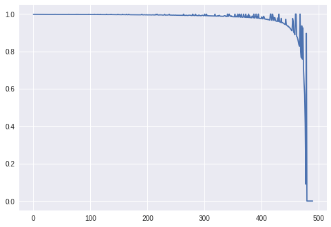
plt.plot(errors)
plt.show()
Although it is really simple it is not stable. When P(X,Y) comes close to 1 my update rules seem to destroy everything. I am going to explore these issues when I am really explaining what I am implementing in the next post.