For human babies we know that:
Depth perception, which is the ability to judge if objects are nearer or farther away than other objects, is not present at birth. It is not until around the fifth month that the eyes are capable of working together to form a three-dimensional view of the world and begin to see in depth.
There are many techniques involved in the depth perception. For example parallax or occlusion. We can divide all of them roughly into the categories of monocular and binocular vision capabilities.
This blog post explain depth estimation of binocular vision systems, camera models and epipolar geometry.
Basic intuition
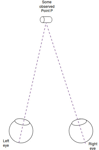
Two eyes/cameras at different locations look at the same object.
How can we determine the distance of the person to the object (“the depth”)?
The simplest answer: We compare the position of an object in the left image to the same object in the right image.
How do we find the object from the left image in the right one?
This is called the correspondence problem. Generally speaking we try to identify areas of the left image which can be found easily in the right image. Obviously that depends on the image. Large homogeneous areas, like the sea, are a problem for this.
But searching the whole image is time intensive, right?
Correct! Epipolar geometry comes in handy here. Given a feature in the left image, we can restrict the search space to a single line in the right image.
If we have found the pixel positions of the same object in the left and the right image, how do we calculate depth?
Knowing the position and orientation of both cameras/eyes does the trick. In the simplest case: we calculate the distance between these pixel features and scale this “disparity” to the real world.
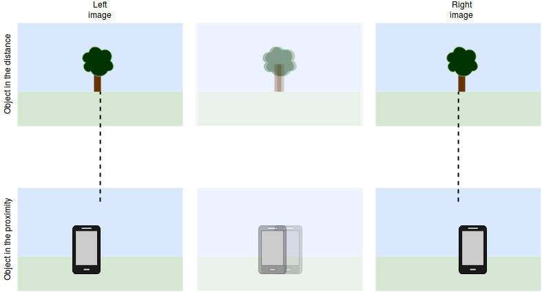
You can experiment with this by closing one eye, focusing an object near you, and then switch the closed eye to the other side. Repeat this with an object in the distance. The distant object moved far less than the one close to you!
Camera model
The relationship between the position on the retina and the position in the real world is necessary to know. When we are talking about cameras instead of eyes the “camera model” provides us with the relationship image plane to real world. Usually we assume to have a simple pinhole camera model without a lens.
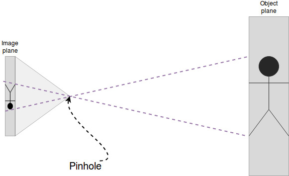
A point P on the object plane has camera coordinates \((x, y, z)\). In automotive vision we call them \((\xi, \eta, \zeta)\) The unit of these coordinates is usually something like millimeters. It does not matter as long as you sty consistent.
The origin of the camera coordinate system is in the focal point of the camera.
In case of the pinhole camera model the focal point is the pinhole therefore the camera coordinate system is originated at the pinhole.
The pinhole camera has an important internal parameter: The focal length is the distance from the focal point to the image plane (The effect of the focal length changes once we use a lens)
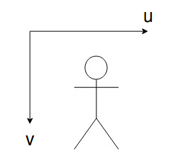
A point (pixel in digital) image plane has the coordinates \((u, v)\) The usually-called y-axis is pointing downwards for historically reasons when images where incrementally built row by row on old television screens.
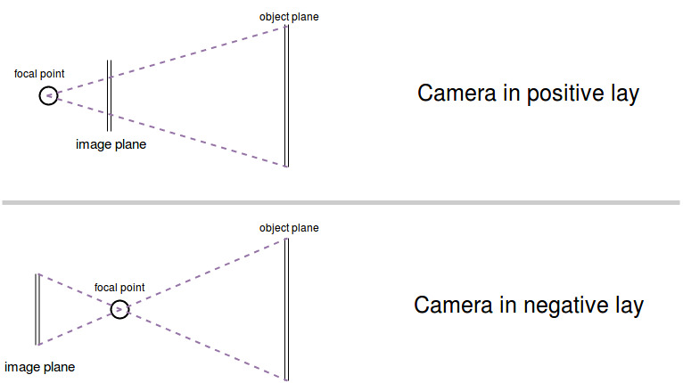
In order to make the calculations a little bit easier it is sometimes preferred to calculate with a camera in positive lay, because the image is not flipped upside down.
After settling the basics we can start to look at the situation. The only thing we have to know about are triangles.
The following image contains a point P. This might be an object we observe. Then there is the focal point F which is now behind the image plane because we are using a camera in positive lay. The shortest line from the focal point through the center of the image plane to the center of the object plane is called the princial or optical axis. It stands orthogonal on both of these planes. The intersection of the image plane and the optical axis is called the principal point.
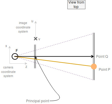
The orthogonality of the optical axis on both planes is important because from that follows that the two triangles are similar.
Figuratively speaking: You can take the large blue triangle “PQF” and scale it down to the red triangle without skewing it.
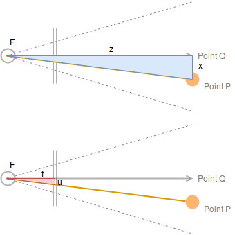
We see:
\[\frac{z}{x} = \frac{f}{u}\]And the same for the y-dimension which is not visible in the diagram:
\[\frac{z}{y} = \frac{f}{v}\]This is the basis for one typical type of math exercise we had at school:
You are standing in front of a tree. Behind the tree you can see the tip of the Eiffel tower. The tree is 10m tall and the Eiffel tower has a height of 300m. Your feet are 8,5m away from the root of the tree. How far away from the Eiffel tower are you?
Let us write the relationships from above in a single vector equation:
\[\frac{z}{x} = \frac{f}{u} \Leftrightarrow \frac{x}{z} = \frac{u}{f} \Leftrightarrow \frac{x \cdot f}{z} = u\] \[\frac{z}{y} = \frac{f}{v} \Leftrightarrow \frac{y}{z} = \frac{v}{f} \Leftrightarrow \frac{y \cdot f}{z} = v\] \[\begin{pmatrix} u \\ v \end{pmatrix} \Leftrightarrow \begin{pmatrix} \frac{x \cdot f}{z} \\ \frac{y \cdot f}{z} \end{pmatrix} \Leftrightarrow \frac{f}{z} \begin{pmatrix} x \\ y \end{pmatrix}\]Let’s try this out on the Eiffel tower example. The Focal point would be the person. The image plane is the tree. So the focal distance is 8,5 meters. We know the tree is 10 m tall which is the value for v. And y=300m.
v = y*f / z <=> 10m = 300m * 8,5m / z <=> z = 300m * 8,5m / 10m <=> z = 255m
This sounds reasonable ;)
But actually the camera coordinates are 3d not 2d. Let’s extend this.
\[\begin{pmatrix} u \\ v \\ f \end{pmatrix} \Leftrightarrow \begin{pmatrix} \frac{x \cdot f}{z} \\ \frac{y \cdot f}{z} \\ \frac{f \cdot z}{z} \end{pmatrix} \Leftrightarrow \frac{f}{z} \begin{pmatrix} x \\ y \\ z \end{pmatrix}\]This is not really what we want because the image coordinates should not store the focal length. But we cannot write this with a scalar product because we want to treat the x and y value different from the z value.
We are looking for a transformation (a matrix):
\[\begin{pmatrix} u \\ v \\ 1 \end{pmatrix} \Leftrightarrow \begin{pmatrix} a1 & a2 & a3 \\ a4 & a5 & a6 \\ a7 & a8 & a9 \end{pmatrix} \begin{pmatrix} x \\ y \\ z \end{pmatrix}\] \[\begin{pmatrix} u \\ v \\ 1 \end{pmatrix} \Leftrightarrow \begin{pmatrix} \frac{f}{z} & 0 & 0 \\ 0 & \frac{f}{z} & 0 \\ 0 & 0 & \frac{1}{z} \end{pmatrix} \begin{pmatrix} x \\ y \\ z \end{pmatrix}\]Intrinsic camera calibration
If we multiply both sides of the equation above with the unknown “z” we can remove the z from the matrix so it only contains internal configuration parameters of the camera (namely f). This is the basic Intrinsic camera calibration K sometimes also referred to as intrinsics only.
\[z \cdot \begin{pmatrix} u \\ v \\ 1 \end{pmatrix} = \begin{pmatrix} f & 0 & 0 \\ 0 & f & 0 \\ 0 & 0 & 1 \end{pmatrix} \begin{pmatrix} x \\ y \\ z \end{pmatrix}\]with: \(K = \begin{pmatrix} f & 0 & 0 \\ 0 & f & 0 \\ 0 & 0 & 1 \end{pmatrix}\)
Inverse: \(K^{-1} = \begin{pmatrix} 1/f & 0 & 0 \\ 0 & 1/f & 0 \\ 0 & 0 & 1 \end{pmatrix}\)
There exists an extension to the basic camera model which allows to move the x- and y-coordinate of the princial point (\(c_x\) and \(c_y\)). And the focal length can be differentiated into a focal length in horizontal (\(f_x\)) and vertical (\(f_z\)).
Extented intrinsic camera calibration:
\[K = \begin{pmatrix} f_x & 0 & c_x \\ 0 & f_y & c_y \\ 0 & 0 & 1 \end{pmatrix}\] \[K^{-1} = \begin{pmatrix} f_x & 0 & -c_x/f_x \\ 0 & f_y & -c_y/f_y \\ 0 & 0 & 1 \end{pmatrix}\]Intrinsics of a real camera:
\[K = \begin{pmatrix} f_x \cdot m_x & \gamma & c_x \\ 0 & f_y \cdot m_y & c_y \\ 0 & 0 & 1 \end{pmatrix}\]\(\gamma\) describes the skew coefficient between the x and y axis. It is zero most of the times. \(m_x\) and \(m_y\) are scaling factors which relate pixels to a distance measure (like millimeters).
Extrinsic camera calibration
The “extrinsics” describe the rotation and translation from the camera coordinate system to the world coordinate system.
The translation t is the difference of the origins (column vector with three entries). The rotation matrix R is a SO(3) matrix. Most of the time they are combined to a homogeneous transformation matrix:
The position and orientation of the camera in the world coordinate system are captured in the following matrix:
\[C = \begin{pmatrix} R \in SO(3) & t \\ 0 ~ 0 ~ 0 & 1 \end{pmatrix}\]Projection matrix
Using the intrinsics and extrinsics we describe the relationship of a pixel on the image plane and a 3d point in the world coordinate system:
\[C^{-1} K^{-1} \begin{pmatrix} u \cdot z \\ v \cdot z \\ z \\ 1 \end{pmatrix} = \begin{pmatrix} x \\ y \\ z \\ 1 \end{pmatrix}\](note that the matrices and vectors have to be extended to be homogeneous)
The same relationship inverted:
\[K C \begin{pmatrix} x \\ y \\ z \\ 1 \end{pmatrix} = \begin{pmatrix} u \cdot z \\ v \cdot z \\ z \\ 1 \end{pmatrix}\]The common appearance of C next to K is captured in the Projection matrix P:
\[P = K C = K [R|t]\]Inverse: \(P^{-1} = (K C)^{-1} = C^{-1} K^{-1}\)
Note: We can determine C and K a priori for a camera system. The only thing that is missing in order to calculate the 3d coordinate in the world is the depth z.
As long as we don’t have the exact z, the mapping is from pixels in the image plane to rays in the world coordinates.
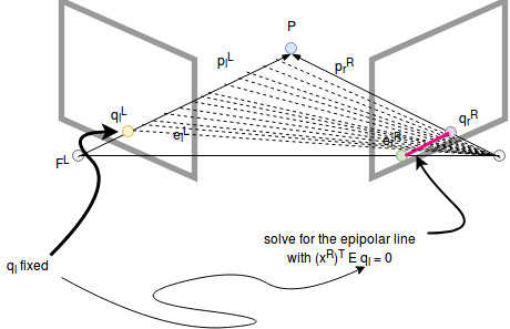
Epipolar geometry
To solve the depth problem (how to estimate the z-value) we introduce a second camera to our setup:
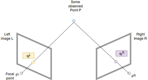
Both cameras observe the same point P. As mentioned in the camera models above they capture the ray from P to their focal points F in the pixel at the coordinate q. A coordinate in the left camera coordinate system is denoted with superscript L, for example \(F^L\), and a coordinate on the left image plane with lowerscript l, for example \(q_{l}^{L}\).
To make the calculations easier we assume the distance from the image planes to their focal points to be 1.
We can draw a vector from \(F^L\) to \(F^R\) which we call the baseline. It captures the positional movement between the two camera centers.
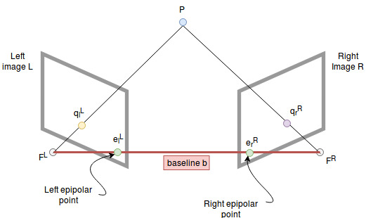
The intersection points of the baseline with the image planes are called epipolar points. The two focal points and the point P span a plane (yellow triangle) which we call the epipolar plane.
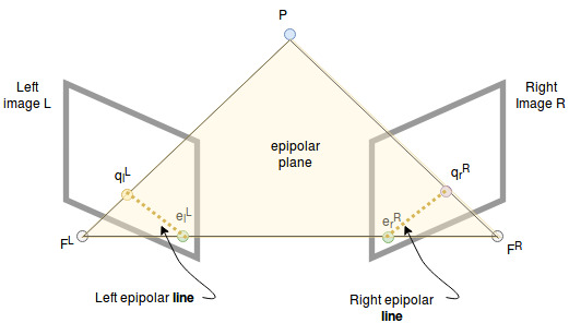
The intersection of this plane with the image planes are called epipolar lines. All 3d points which lie on the triangle are projected onto these lines.
Central relationship
The baseline, the left arm (\(\vec{p_l^L}\)) and the right arm (\(\vec{p_r^R}\)) of the triangle lie on the same plane. From that follows, that a vector which stands orthogonal on the left arm and the baseline (fat red arrow) also stand orthogonal on the right arm!
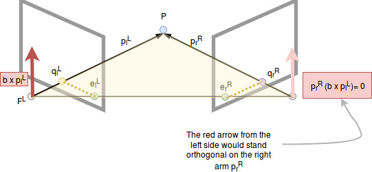
Note that this equality only holds in one of the camera coordinate systems (either one is good) but not if the vectors are represented in different ones.
\(\vec{p}_r^L\) is the right arm expressed in the left coordinate system. We want to transform this to the right coordinate system.
Transform right arm from left to right coordinate system
This is how x in the right coord. system can be descibed in the left camera coordinate system: \(\vec{x}^L = D \vec{x}^R + \vec{b}^L\)
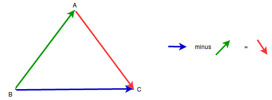
\(\vec{p_r^L}\) can be expressed as the connection between two points:
\[\vec{p_r^L} = \vec{(F_rP)}^L = -\vec{(PF_r)}^L \\\]Rewrite the right arm as the difference between the left arm and the baseline.
Plug into the defintion of \(\vec{p_r^L} = \vec{(F_rP)}^L = -\vec{(PF_r)}^L\):
\[-\vec{(PF_r)}^L = -( \vec{(F_lF_r)}^L - \vec{(F_lP)}^L) = \\ -\vec{(F_lF_r)}^L + \vec{(F_lP)}^L = \\ \vec{(F_lP)}^L - \vec{(F_lF_r)}^L\]Long story short: The right side is the difference between the left side and the baseline.
\[\vec{p_r^L} = \vec{(F_lP)}^L - \vec{(F_lF_r)}^L\]Now we transform this to the right coordinate system with: \(\vec{x}^L = D \vec{x}^R + \vec{b}^L\)
\[\vec{p_r^L} = \vec{(F_lP)}^L - \vec{(F_lF_r)}^L = \\ D \vec{(F_lP)}^R + \vec{b}^L - D \vec{(F_lF_r)}^R + \vec{b}^L = \\ D \vec{(F_lP)}^R - D \vec{(F_lF_r)}^R = \\ D (\vec{(F_lP)}^R - \vec{(F_lF_r)}^R) \\\]In the last line we have \(\vec{(F_lP)}^R - \vec{(F_lF_r)}^R\) now both in the right coordinate system. Which means that this is just \(\vec{p}_r^R\)!
\[D (\vec{(F_lP)}^R - \vec{(F_lF_r)}^R) = \\ D \vec{p}_r^R\]Note that we got rid of the baseline.
Apply to central relationship:
\[D \vec{p}_r^R \cdot (\vec{b}^L \times \vec{p}_l^L)= 0\]Substitute world point by image points
As we have seen in the camera model, a given pixel on the image plane captures a whole ray that goes through it to the focal point.
Mathematically this means that the ray has one dimension more than the pixel. This additional dimension is \(z\).
Therefore we have gotten the following relationship between a point in the camera coordinate system and on the image plane (focal length = 1):
\[q_l = \frac{f}{z_l^L} \vec{p}_l^L = \frac{1}{z_l^L} \vec{p}_l^L \Leftrightarrow \\ \vec{p}_l^L = q_l \cdot z_l^L\]and for the right side of the triangle:
\[q_r = \frac{1}{z_r^R} \vec{p}_r^R \Leftrightarrow \\ \vec{p}_r^R = q_r \cdot z_r^R\]Essentially we are using the simplest intrinsic camera matrix in order to project the point P to the image plane in the equation:
\[D \vec{p}_r^R \cdot (\vec{b}^L \times \vec{p}_l^L) = 0 \Leftrightarrow \\ D (q_r \cdot z_r^R) \cdot (\vec{b}^L \times (q_l \cdot z_l^L)) = 0\]Because z is in both coordinate systems just a positive number, we can factor it out and it gets removed from both sides of the equation.
\[(q_r)^T D^T \cdot (\vec{b}^L \times q_l) = 0\]Cross product as matrix
We can write the cross product with a given vector \(\vec{b}_L\) as a matrix multiplication:
\[\vec{b}^L \times q_l = \begin{pmatrix} 0 & -b_z^L & b_y^L \\ b_z^L & 0 & -b_x^L \\ -b_y^L & b_x^L & 0 \end{pmatrix} q_l = [b^L] _ {\times} q_l\]Insert this into the central relationship:
\[(q_r)^T D^T \cdot [b^L] _ {\times} q_l = 0\]Essential matrix
The rotation matrix D and the new matrix \([b^L] _ {\times}\) are called the Essential Matrix: \(E = D^T [b^L] _ {\times}\)
Note: E only contains the geometric parameters of the binocular camera system. Which are the baseline and the rotation matrix D.
Insert this into the central relationship:
\[(q_r)^T E q_l = 0\]Epipolar lines
And now we can clearly see that E is constant and only \(q_l\) and \(q_r\) are variables. Suppose \(q_l\) was known, then the central relationship becomes a function of \(q_r\): The epipolar line of the right image plane.
The same works in the other direction.
Note: If we pick a point in one image we only have to search on the epipolar line of the other image to find the corresponding point if it is visible.
Epipoles: As initially stated the epipolar line can be drawn through q and the epipole. This can be shown with the equation above.
Fundamental matrix
Instead of calculating with camera coordinates q we want to calculate with image coordinate (u,v). Let’s modify the essential matrix to fix this. Every camera gets a matrix of intrinsic parameters \(A_l\) and \(A_r\). Remember that so far the focal length was 1 and we had no scaling factors in use.
Fundamental matrix F:
\[F = A_r^{-T} E A_l^{-1}\]Central relationship with Fundamental matrix F:
\[(u_r, v_r, 1) F \begin{pmatrix} u_l \\ v_l \\ 1 \end{pmatrix} = 0\]There are two ways to obtain the fundamental matrix:
- Calculate it from the geometric relations and intrinsic of the cameras
- Or use the “8 point algorithm” to estimate it
Simplified setup
After a process called rectification (see below) we get to a simpler setup. Actually we can also try to setup our cameras initially like this (for example in cars).
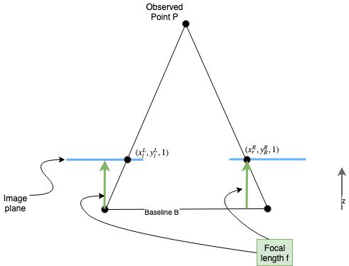
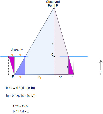
There are two equal triangles (red) which capture the relationship between the same point in the left and in the right camera image. The length of the yellow sides of the triangles are the same proportional to each others. The right triangle only has a yellow dot because the line has a length of zero in this image.
This is the relationship we humans “feel”: The closer the object the larger the disparity on the image plan.
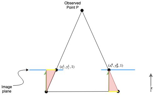
This relationship can also be found in the baseline of the small triangle in the following image. Note the equal triangles!
General possibility for depth estimation: Calculate the disparity which is the baseline for the smaller triangle: \(d = x_l - (x_r - b)\). The \((x_r - b)\) means to move the red dot from the right to the left (see next image).
The ratio between the left and the right part of this smaller baseline is the same as for the bigger baseline: \(\frac{b_l}{b} = \frac{x_l}{d}\)
That’s how we get: \(b_l = b \cdot \frac{x_l}{d}\)
Because the triangles have the same ratios… \(\frac{f}{x_l} = \frac{z}{b_l}\)
… we can calculate the depth \(z = \frac{b_l \cdot f}{x_l}\)
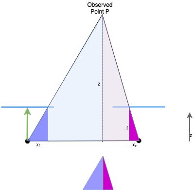
Correct derivation:
Find the intersection of the left and right arm. With the correct scaling factor \(\lambda_l\) the image point \(q_l\) becomes P:
\[\begin{equation} \begin{split} \begin{bmatrix} p_x^L \\ p_y^L \\ p_z^L \end{bmatrix} &= \lambda_l \cdot \begin{bmatrix} x_l^L \\ y_l^L \\ 1 \end{bmatrix} \\ \end{split} \end{equation}\]We express the right arm of the triangle also in the left coordinate system:
\[\begin{equation} \begin{split} \begin{bmatrix} x_r^L \\ y_r^L \\ z_r^L \end{bmatrix} &= \begin{bmatrix} b \\ 0 \\ 0 \end{bmatrix} + \overrightarrow{F_r^Rq_r^R} \\ \begin{bmatrix} x_r^L \\ y_r^L \\ z_r^L \end{bmatrix} &= \begin{bmatrix} b \\ 0 \\ 0 \end{bmatrix} + (q_r^R - F_r^R) \\ \begin{bmatrix} x_r^L \\ y_r^L \\ z_r^L \end{bmatrix} &= \begin{bmatrix} b \\ 0 \\ 0 \end{bmatrix} + ( \begin{bmatrix} x_r^R \\ y_r^R \\ 1 \end{bmatrix} - \begin{bmatrix} 0 \\ 0 \\ 0 \end{bmatrix} ) \\ \begin{bmatrix} x_r^L \\ y_r^L \\ z_r^L \end{bmatrix} &= \begin{bmatrix} b \\ 0 \\ 0 \end{bmatrix} + \begin{bmatrix} x_r^R \\ y_r^R \\ 1 \end{bmatrix} \\ \begin{bmatrix} x_r^L \\ y_r^L \\ z_r^L \end{bmatrix} - \begin{bmatrix} b \\ 0 \\ 0 \end{bmatrix} &= \begin{bmatrix} x_r^R \\ y_r^R \\ 1 \end{bmatrix} \\ \begin{bmatrix} x_r^L - b \\ y_r^L \\ z_r^L \end{bmatrix} &= \begin{bmatrix} x_r^R \\ y_r^R \\ 1 \end{bmatrix} \\ \end{split} \end{equation}\]With that we can find the same point P with the right arm of the triangle
\[\begin{equation} \begin{split} \begin{bmatrix} p_x^L \\ p_y^L \\ p_z^L \end{bmatrix} &= \begin{bmatrix} b \\ 0 \\ 0 \end{bmatrix} + \lambda_r \cdot \begin{bmatrix} x_r^L - b\\ y_r^L \\ 1 \end{bmatrix} \\ \end{split} \end{equation}\]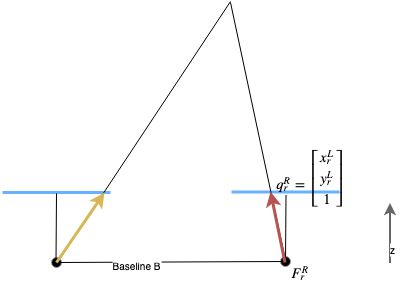
Now we know that both lines should intersect at P. So we solve for this point by setting the two line equations equal:
\[\begin{equation} \begin{split} \lambda_l \cdot \begin{bmatrix} x_l^L\\ y_l^L \\ 1 \end{bmatrix} &= \begin{bmatrix} b \\ 0 \\ 0 \end{bmatrix} + \lambda_r \cdot \begin{bmatrix} x_r^L - b\\ y_r^L \\ 1 \end{bmatrix} \\ \end{split} \end{equation}\]This yields a linear equation system:
- \[\lambda_l x_l^L = b+ \lambda_r \cdot (x_r^L - b)\]
- \[\lambda_l y_l^L = \lambda_r \cdot y_r^L\]
- \[\lambda_l = \lambda_r\]
Replacing the right lambda in (2) with the result from equation (3):
\[\lambda_l y_l^L = \lambda_l \cdot y_r^L \Rightarrow \\ y_l^L =y_r^L\]This is not surprising due to the results from epipolar geometry.
Now replacing the right lambda in (1) with the result from equation (3):
\[\begin{equation} \begin{split} \lambda_l x_l^L &= b+ \lambda_l \cdot (x_r^L - b) \\ x_l^L &= \frac{b}{\lambda_l}+ x_r^L - b \\ x_l^L - x_r^L + b &= \frac{b}{\lambda_l} \\ \frac{x_l^L - x_r^L + b}{b} &= \frac{1}{\lambda_l} \\ \frac{b}{x_l^L - x_r^L + b} &= \lambda_l \\ \end{split} \end{equation}\]Next: We use the replacement from before, that \(x_r^L - b = x_r^R\):
\[\begin{equation} \begin{split} \lambda_l &= \frac{b}{x_l^L - x_r^R} \\ \end{split} \end{equation}\]Last step: Transform to image coordinates by using \(\alpha'\) called the effective focal length, which maps camera coordinates to image plane coordinates (pixels):
- \[u_l = \alpha' \cdot x_l^L + u_0\]
- \[u_r = \alpha' \cdot x_r^r + u_0\]
\(u_0\) is the position of the principal point.
\[\begin{equation} \begin{split} \lambda_l &= \frac{b \alpha'}{u_l - u_r} \\ \end{split} \end{equation}\]Result:
\[\begin{equation} \begin{split} \begin{bmatrix} p_x^L \\ p_y^L \\ p_z^L \end{bmatrix} &= \frac{b \alpha'}{u_l - u_r} \cdot \begin{bmatrix} x_l^L \\ y_l^L \\ 1 \end{bmatrix} \end{split} \end{equation}\]With disparity \(d = u_l - u_r\) .
Image rectification
In reality we can’t manufacture such a ideal camera setup. Therefore we change the images of our setup by a process called image rectification in order to align to a virtual camera setup which have the same focal length, are aligned perfectly and whose focal points match the original ones.
Procedure:
- Find common camera intrinsics A’ (for example by taking the average of the original intrinsics \(A_l\) and \(A_r\) of the left and right camera)
- Find the common coordinate systems for both cameras, so that the x-axis lie parallel to the baseline
- Find the rotation matrices \(D_l\) and \(D_r\) which rotate the camera coordinate systems to their common coordinate systems.
- Transform the original camera images to rectified images which could have been captured from the virtual cameras
In the pinhole camera model we know the relationship between the intrinsics, the point p and the pixels.
\[\begin{equation} \begin{split} A_l \cdot \vec{p} &= p_z \begin{pmatrix} u \\ v \\ 1 \end{pmatrix}\\ \vec{p} &= A_l^{-1} \cdot p_z \begin{pmatrix} u \\ v \\ 1 \end{pmatrix}\\ \end{split} \end{equation}\]We know that the relationship stays but the pixels change after rectification:
\[\begin{equation} \begin{split} A' \cdot \vec{p}' &= p_z' \begin{pmatrix} u' \\ v' \\ 1 \end{pmatrix}\\ \end{split} \end{equation}\]p’ is \(\vec{p}\) but rotated using \(D_l\) into the new camera coordinate system:
\[\begin{equation} \begin{split} A' \cdot D_l \vec{p} &= p_z' \begin{pmatrix} u' \\ v' \\ 1 \end{pmatrix}\\ \end{split} \end{equation}\]Now plug in the original definition of point p:
\[\begin{equation} \begin{split} A' \cdot D_l \cdot A_l^{-1} \cdot p_z \begin{pmatrix} u \\ v \\ 1 \end{pmatrix} &= p_z' \begin{pmatrix} u' \\ v' \\ 1 \end{pmatrix}\\ \underbrace{A' \cdot D_l \cdot A_l^{-1}}_\textrm{A priori knowledge} \begin{pmatrix} u \\ v \\ 1 \end{pmatrix} &= \frac{p_z'}{p_z} \begin{pmatrix} u' \\ v' \\ 1 \end{pmatrix}\\ \end{split} \end{equation}\]Having figured out all of the a priori knowledge we can calculate the left hand side. Imagine the result was \((a, b, c)^T\):
\[\begin{equation} \begin{split} \begin{pmatrix} a \\ b \\ c \end{pmatrix} &= \frac{p_z'}{p_z} \begin{pmatrix} u' \\ v' \\ 1 \end{pmatrix}\\ \end{split} \end{equation}\]Then we can solve for \(u'\) and \(v'\) by diving the relevant entry (\(a\) or \(b\)) by c because c is only the missing factor \(\frac{p_z'}{p_z}\):
\(u' = a/c\) and \(v' = b/c\).
(gemeinfrei)