GTSRB with Keras
In my last blog post I described how I built a model for traffic sign recognition with tensorflow. The data set contains 43 different German traffic signs:
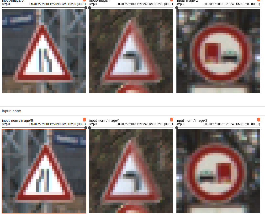
It is made out of 39.000 training images and the 12.000 images for testing.
To use the network in a browser application I wanted to “deploy” it via tensorflow.js! (https://www.youtube.com/watch?v=656l4IfhM10)
The easiest way to use a pretrained model in tensorflow.js seems to be by using Keras (pip install keras). Keras is a high-level API which can use multiple backends, with tensorflow and tensorflow.js being part of them.
Because I still don’t have a GPU I am going to try to work with colab.research.google.com which provides the same convenience as the Kaggle notebooks coming with access to one GPU.
Data Set Source: http://benchmark.ini.rub.de/?section=gtsrb&subsection=dataset
Inspirational blog entry: keras tutorial
Loading the data
As a first step I have to write some code to download the dataset into the notebook.
import requests
import os.path
import zipfile
import os


# Load the dataset
train_data_url = 'http://benchmark.ini.rub.de/Dataset/GTSRB-Training_fixed.zip'
test_data_url = 'http://benchmark.ini.rub.de/Dataset/GTSRB_Final_Test_Images.zip'
test_data_classes = 'http://benchmark.ini.rub.de/Dataset/GTSRB_Final_Test_GT.zip'

def maybe_download_file(url):
  # the name of the file
  local_filename = url.split('/')[-1]
  if os.path.isfile(local_filename):
    print('File already exists')
    return local_filename
  # NOTE the stream=True parameter
  r = requests.get(url, stream=True)
  with open(local_filename, 'wb') as f:
      for chunk in r.iter_content(chunk_size=1024):
          if chunk: # filter out keep-alive new chunks
              f.write(chunk)
              #f.flush() commented by recommendation from J.F.Sebastian
  return local_filename


def extract_archive(file_name, target_dir):
  # only extract the zip if the target_dir doesn't exist
  if os.path.isfile(target_dir):
      print('Dir already exists')
      return target_dir
  with open(file_name, 'rb') as f:
      zf = zipfile.ZipFile(f)
      zf.extractall(target_dir)
  return target_dir


file_path = maybe_download_file(test_data_url)
extract_archive(file_path, 'test_data')

file_path = maybe_download_file(train_data_url)
extract_archive(file_path, 'train_data')

file_path = maybe_download_file(test_data_classes)
extract_archive(file_path, 'train_data_labels')
The code downloads the training and testing data sets and extracts them to the folders “test_data”, “train_data” and “train_data_labels”.
The following function is a python version of the unix commandline tool tree which outputs a nice looking overview over the files in a directory until some depth.
def list_files(startpath, depth=3):
  for root, dirs, files in os.walk(startpath):
      level = root.replace(startpath, '').count(os.sep)
      if level <= depth:
        indent = ' ' * 4 * (level)
        print('{}{}/'.format(indent, os.path.basename(root)))
        subindent = ' ' * 4 * (level + 1)
        for f in files:
            print('{}{}'.format(subindent, f))


list_files('.', depth=3)
This is the shortened output:
./
    GTSRB_Final_Test_GT.zip
    GTSRB-Training_fixed.zip
    GTSRB_Final_Test_Images.zip
    test_data/
        GTSRB/
            Readme-Images-Final-test.txt
            Final_Test/
                Images/
                    GT-final_test.test.csv
    train_data/
        GTSRB/
            Training/
                Readme.txt
                00002/
                    GT-00002.csv
                00031/
                    GT-00031.csv

		[...]
    train_data_labels/
        GT-final_test.csv
Install requirements
!pip install keras
!pip install scikit-image
The ! in the beginning of a line allows us to execute shell commands from within a notebook.
Preprocessing the images
As already mentioned in my previous blog post, the images must be cropped before using them.
import numpy as np
import os
import glob

from skimage import io, transform

NUM_CLASSES = 43
IMG_SIZE = 32

def get_class(img_path):
    "Use the directory name to get the class number"
    return int(img_path.split('/')[-2])

# The folder where the training data ist located
root_dir = 'train_data/GTSRB/Training/'
imgs = []
labels = []

# Get all images and shuffle them
all_img_paths = glob.glob(os.path.join(root_dir, '*/*.ppm'))
np.random.shuffle(all_img_paths)

for i, img_path in enumerate(all_img_paths):
    if i%1000 == 0:
        print("{}".format(i))
    # read the image and crop it
    img = preprocess_img(io.imread(img_path))
    label = get_class(img_path)
    imgs.append(img)
    labels.append(label)

X = np.array(imgs, dtype='float32')
# Make one hot targets
Y = np.eye(NUM_CLASSES, dtype='uint8')[labels]
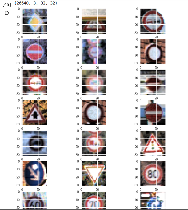
A glimpse into the data set
Now that we have the images in the RAM we should take a look at them in order to check whether they are okay.
%matplotlib inline

# Visualize some images
n_images_per_class = 3

import random
import numpy as np
import matplotlib.pyplot as plt

w=IMG_SIZE
h=IMG_SIZE

fig=plt.figure(figsize=(10, 80))

columns = n_images_per_class
rows = NUM_CLASSES

print(X.shape)

for i in range(1, columns*rows +1):
  img = imgs[random.randint(0, 26640)]
  img = np.rollaxis(img, -1)
  img = np.rollaxis(img, -1)
  fig.add_subplot(rows, columns, i)
  plt.imshow(img)

plt.show()
Building a CNN with Keras
Keras is being build and maintained by Francois Chollet at Google. Lots of information can be found at blog.keras.io.
It is a deep learning library for Python which abstracts the implementation details of its backends to export a user friendly API.
from keras.models import Sequential
from keras.layers.core import Dense, Dropout, Activation, Flatten
from keras.layers.convolutional import Conv2D
from keras.layers.pooling import MaxPooling2D
from keras.optimizers import SGD
from keras import backend as K

# Check if the GPU is used
print(K.tensorflow_backend._get_available_gpus())

# Whether the format is
# - "channels_last" (IMAGE_SIZE, IMAGE_SIZE, 3) or
# - "channels_first" (3, IMAGE_SIZE, IMAGE_SIZE)
K.set_image_data_format('channels_last')


dropout_rate = 0.4
l2 = 0.01
l1 = 0.01


def cnn_model():
    model = Sequential()

    model.add(Conv2D(32, (3, 3), padding='same',
                     input_shape=(IMG_SIZE, IMG_SIZE, 3),
                     activation='relu'
                    ))
    model.add(Conv2D(32, (3, 3), activation='relu',
                     kernel_regularizer=regularizers.l2(l2)))
    model.add(MaxPooling2D(pool_size=(2, 2)))
    model.add(Dropout(dropout_rate))

    model.add(Conv2D(64, (3, 3), padding='same',
                     activation='relu'))
    model.add(Conv2D(64, (3, 3), activation='relu'))
    model.add(MaxPooling2D(pool_size=(2, 2)))
    model.add(Dropout(dropout_rate))

    model.add(Conv2D(128, (3, 3), padding='same',
                     activation='relu'))
    model.add(Conv2D(128, (3, 3), activation='relu'))
    model.add(MaxPooling2D(pool_size=(2, 2)))
    model.add(Dropout(dropout_rate))

    model.add(Flatten())
    model.add(Dense(512, activation='relu',
                     kernel_regularizer=regularizers.l2(l2)
                     #activity_regularizer=regularizers.l1(l1)
        ))
    model.add(Dropout(dropout_rate))
    model.add(Dense(NUM_CLASSES, activation='softmax'))
    return model
It is even easier to build any “sandwich” with keras and under the hood you get the ability to run the tensorflow gpu operations.
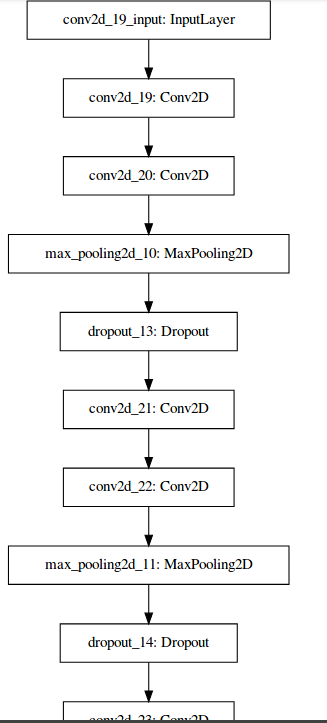
The model can be visualized with the following code (I had to restart my kernel after installing pydot):
# install pydot
!pip install pydot
!apt-get install graphviz

from IPython.display import SVG
from keras.utils.vis_utils import model_to_dot

SVG(model_to_dot(model).create(prog='dot', format='svg'))
Training
from keras.optimizers import SGD

model = cnn_model()

# let's train the model using SGD + momentum
lr = 0.01
sgd = SGD(lr=lr, decay=1e-6, momentum=0.9, nesterov=True)
model.compile(loss='categorical_crossentropy',
              optimizer=sgd,
              metrics=['accuracy'])

from keras.callbacks import LearningRateScheduler, ModelCheckpoint


def lr_schedule(epoch):
    return lr * (0.1 ** int(epoch / 10))

batch_size = 32
epochs = 10

model.fit(X, Y,
          batch_size=batch_size,
          epochs=epochs,
          validation_split=0.2,
          callbacks=[LearningRateScheduler(lr_schedule),
                     ModelCheckpoint('model.h5', save_best_only=True)]
          )
The network is able to achieve a fitness of above 98% on the training data…
Evaluate
Let’s see how far we can go on new images (the test data):
import pandas as pd

# train_data_labels/
#         GT-final_test.csv

# test_data/
#        GTSRB/
#            Readme-Images-Final-test.txt
#            Final_Test/
#                Images/
#                    GT-final_test.test.csv


test = pd.read_csv('train_data_labels/GT-final_test.csv', sep=';')

# Load test dataset
X_test = []
y_test = []
i = 0
for file_name, class_id in zip(list(test['Filename']), list(test['ClassId'])):
    img_path = os.path.join('test_data/GTSRB/Final_Test/Images/', file_name)
    X_test.append(preprocess_img(io.imread(img_path)))
    y_test.append(class_id)

X_test = np.array(X_test)
y_test = np.array(y_test)

# predict and evaluate
y_pred = model.predict_classes(X_test)
acc = np.sum(y_pred == y_test) / np.size(y_pred)
print("Test accuracy = {}".format(acc))
Test accuracy = 0.8463182897862233
That is amazing for that little effort compared to my results using the tensorflow layers API. It looks like I need a lot more practice with tensorflow…
After playing around with the parameters I achieved 85% accuracy with the following settings:
- batch size: 128
- epochs: 30
- dropout: 40%
- learning_rate: exponential decay
- optimization with SGD nesterov momentum(0.9) decay=1e-6
- L2 regularization on the dense layer with 512 inputs
Export for further use
The model’s weights are already stored in a “model.h5” but to use it with tensorflow.js to make the network usable in the browser we can run the following code snippet:
# install tensorflow for javascript python package
! pip install tensorflowjs

import tensorflowjs as tfjs
import shutil

model_dir = 'tfjs'
model_zip = 'keras_model.zip'

# create the directory {model_dir}
if not os.path.exists(model_dir):
  os.mkdir(model_dir)

# save the model to that dir
tfjs.converters.save_keras_model(model, model_dir)

# function to zip a folder
def zipdir(path, ziph):
    # ziph is zipfile handle
    for root, dirs, files in os.walk(path):
        for file in files:
            ziph.write(os.path.join(root, file))

# if a zip file with the name {model_zip} already exists
# -> delete it
if os.path.exists(model_zip):
  os.remove(model_zip)

# zip the folder
with zipfile.ZipFile(model_zip, 'w') as zipf:
    zipdir(model_dir, zipf)
    zipf.close()

# this is code to download the zip file from the google colab notebook
from google.colab import files
files.download(model_zip)
The next blog post will show how load the model with tensorflow.js, upload an image and get a prediction.