This post aims to give an overview of Sum-Product Networks with a graphical explanation. It also contains an introduction on inference.

TL;DR Sum-Product Network is a group of probabilistic graphical models with the nice property that inference is linear in time to the size of the network. They consist only of univariate distributions, sums and products.

Introduction

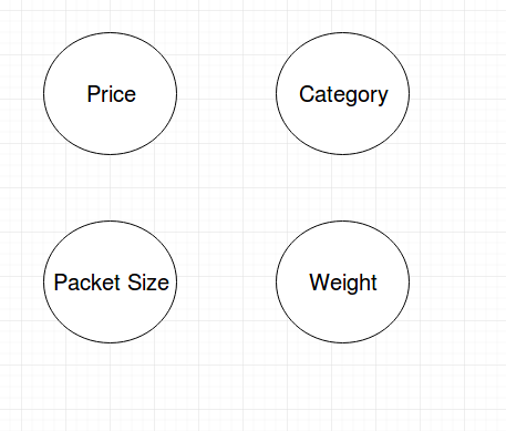
We start with a toy example: Imagine you own a web shop and the products you are selling have the following attributes:

• Price P: {$, \(,\)$}
• Category C: {tech, clothes, stuff}
• Packet size S: {s, m, l}
• Weight W: {light, heavy}

You noticed this customer Joe. He really bought a lot of stuff. A quick report gives you a list of items he bought by their attributes:

Name	Price	Category	Packet Size	Weight
Notebook	$$$	tech	m	heavy
Docking Station	$$	tech	s	light
Monitor	$$	tech	xl	heavy
Smartphone	$$	tech	s	light
Star Wars Shirt	$	clothes	m	light
Light sabor	$	stuff	s	light
Lego Star Wars	$$$	stuff	m	heavy

Now you are wondering: Which of my other products should I advertise to Joe?

You take a look into you inventory: What are the non-sellers?

Name	Price	Category	Packet Size	Weight	P(Joe buys it)
Graphics Card	$$$	tech	m	light	???
Star Wars Fan Art	$$	stuff	xl	heavy	???

The questions we try to answer: Which non-seller should we advertise? Can we calculate a probability that Joe is going to buy a product? If we are restricted to send small packets what should we advertise?

SPN

Probability

Let’s assume that Price P, Category C, Packet Size S and Weight W are random variables. We assume that there is a joint probability distribution f(P, C, S, W) over them. Our target is to approximate this function f by maximizing the likelihood of Joe’s buying history.

Imagine we had a pool of approximations of the original function f. The approximations are called hypothesis h. Together the pool is called the hypothesis space H.

We are looking for the hypothesis h which has the highest probability of producing the buying history of Joe which we are going to call our training data.

\[h_{ML} = arg_{h} max P(training data | h) \cdot P(h)\]

Probabilistic Graphical Model

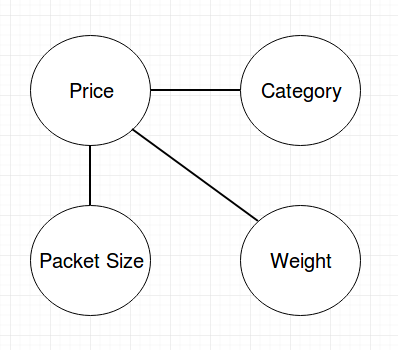
In these models we draw a vertex in a graph for every random variable and an edge to represent some kind of causality (Bayesian Network) or correlation (Markov Network).

Advantages of these models are that they are interpretable and you can combine data with a-priori knowledge. In our case, we know that the price depends on the Packet Size and the Weight because our fulfillment partner charges differently for packets. And the second information: The category influences all of the other variables.

In a Markov Network these dependencies add edges between the vertices:

You can imagine, that in real world scenarios these networks get huge because products could have a lot of attributes and there are multiple levels on influencing. Inference in these graphs is in general NP-complete. The same property holds for Bayesian Networks. Because of that, they are called intractable.

This is the problem where Sum-Product Networks come to rescue.

SPN Idea

We want to build a probabilistic graphical model which only contains univariate distributions, sums and products. The sums can be interpreted as mixtures/clusterings whereas the products have the interpretation of a “part of” relationship.

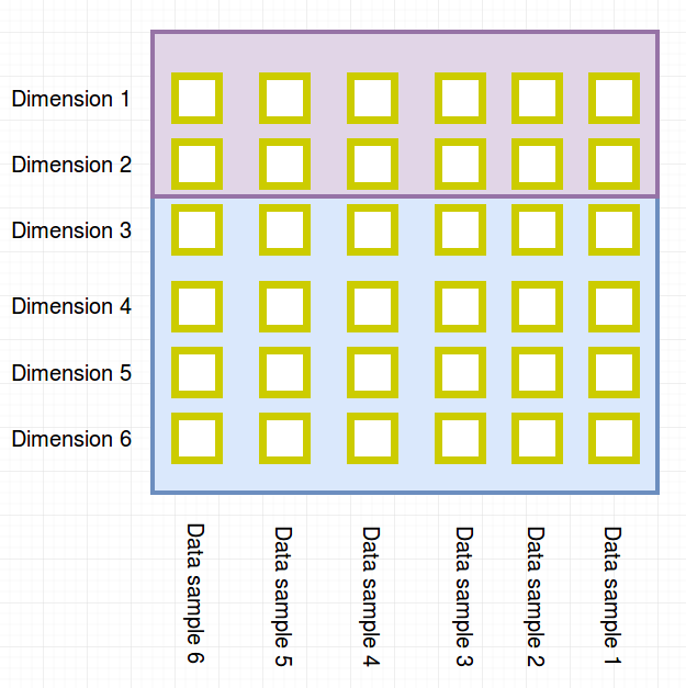
We can illustrate the training data with the dimsions on the y-axis and the samples on the x-axis in the following plot:

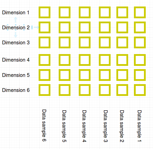
A univariate distribution models the probabilities of “rectangles in a row”: For example the three data points in dimension 3 could be modeled by a binomial distribution.

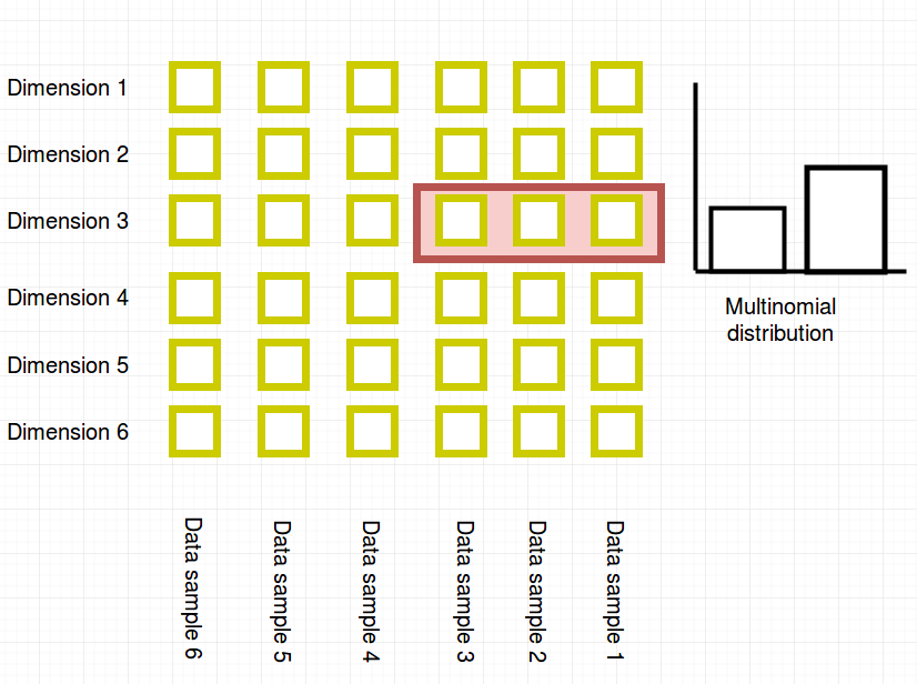
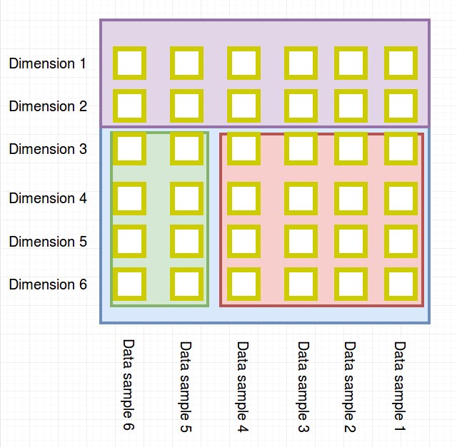
A product node can be visualized as a partitioning of dimensions. In the toy example this will be the three attributes {price, size, weight} seperated from {category}.

A sum node signifies a paritioning of the data points (in the following toy example this could be Amazon’s data (red) and your shop’s data (green)):

Rules SPN

The definition of SPNs is recursive.

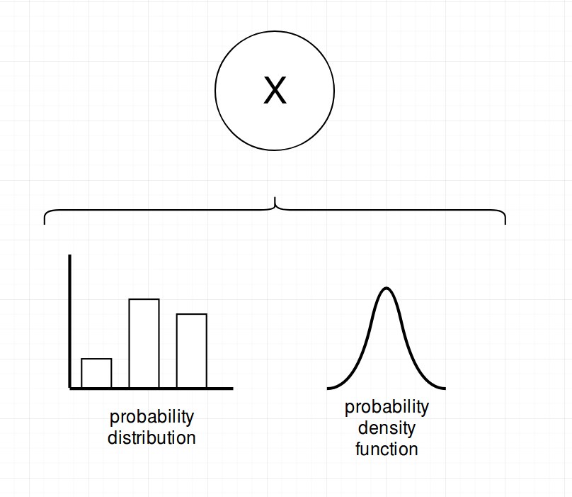
First: A SPN can be any univariate distribution

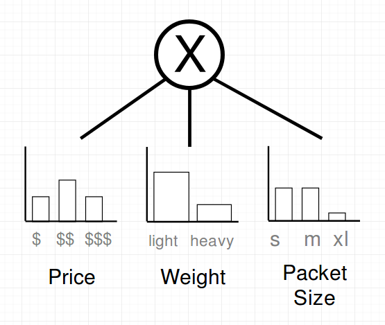
Second: A product over disjunct variables is a SPN

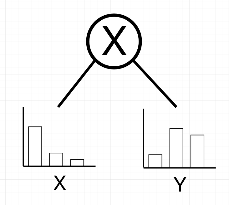
(the big X refers signifies a product)

Third: A weighted sum of SPNs over the same variables is an SPN

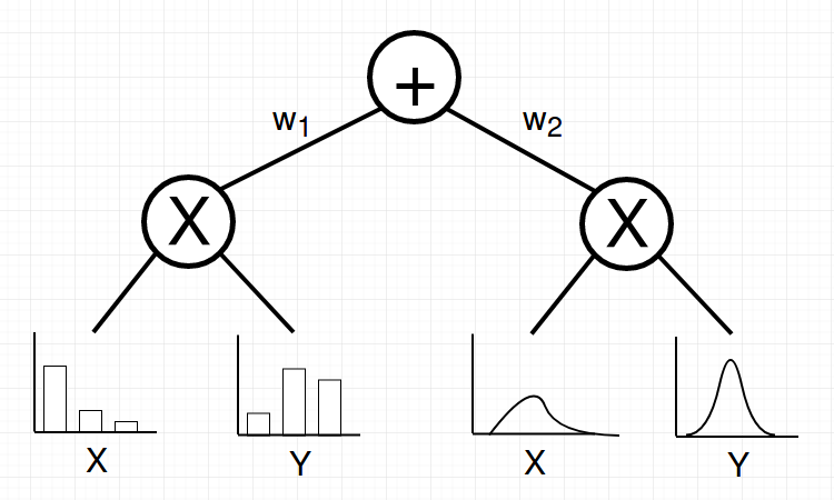
SPN Toy Example

Let’s assume a SPN for the toy example just walked into our office and looks as follows:

And luckily you know a lot of people, so you asked Jeff Bezos about the same attributes of the buying history of Joe’s Amazon Account. Know you have two SPNs which can be combined in a weighted sum to build a bigger SPN. Amazon has a lot more data so you trust their data more, therefore you put a weight of 80% on their subtree.

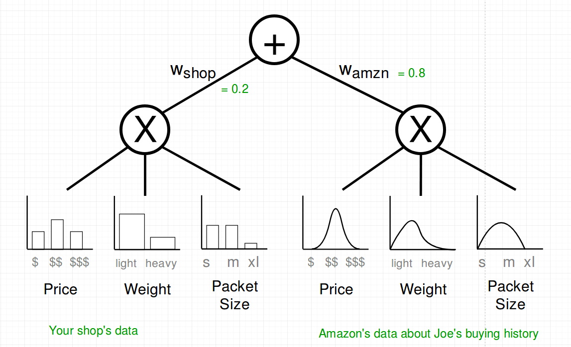
Additionally Amazon provided you with the parametric estimators for the attributes. That should be okay with SPN.

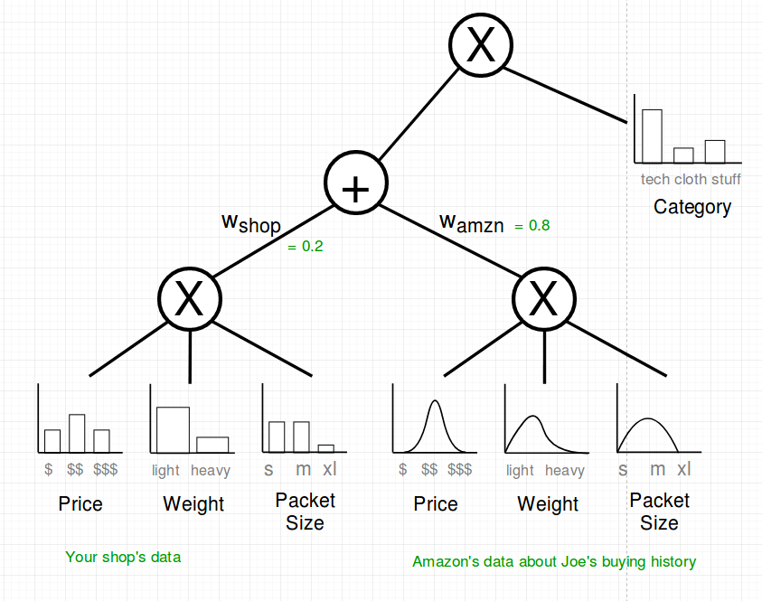
Last step: You add the category variable of which you know that it influences all of the others.

Is this really a probability distribution?

There are two properties that have to be assured in order for a SPN to be a valid distribution:

1. Completeness: The children of sum-nodes have the same scope*
2. Consistency: The children of product-nodes have disjunct scopes*

• What is a scope?: The scope is the set of random variables that is reachable from the node to the leaves.

Let us check the completeness: There is only one sum node and the scope of both children is: {Price, Weight, Packet Size}

What about consistency? The amazon and shop product node have the same children. And all of them are disjunt. For example the scope of Price is {Price} which is disjunct with the scope of Weight which is {Weight}.

The root is also consistent because: {Price, Weight, Packet Size} ∩ {Category} = {} => disjunct

Advantages

Now that we have a SPN, what is it good for?

All Marginals Are Computable in Linear Time

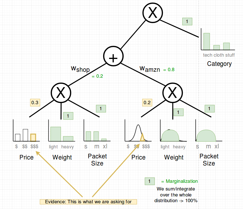
Example: What is the probability of P(Price=$$$) ?

Therefore we marginalize all other variables we are not interested right now. Which means that their probability is 100%.

And we select the probability of the variable price at “high” ($$$).

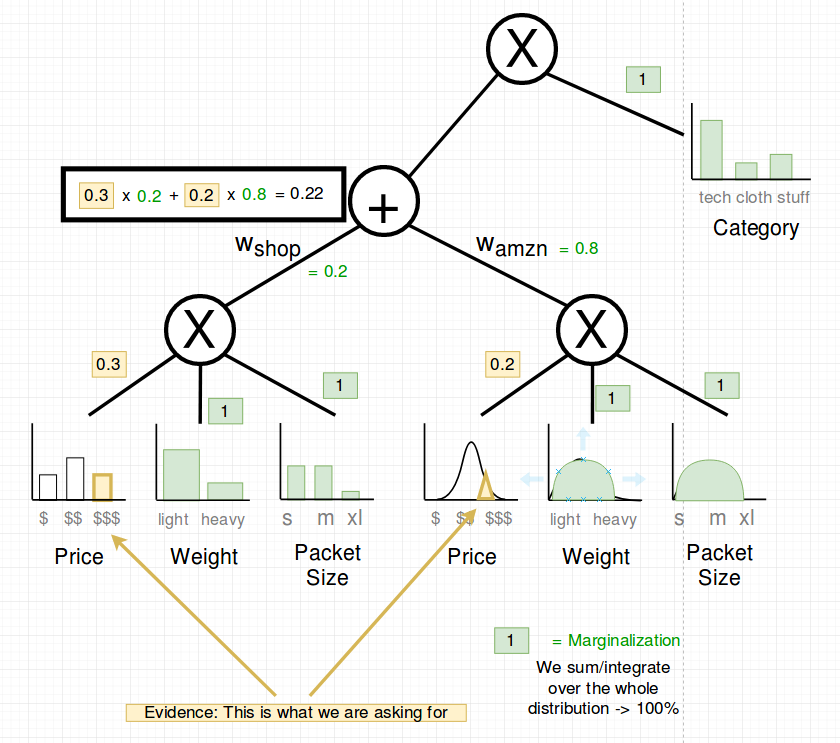
Now we propagate up to the sum node.

The last propagation to the root is multiplication with 1.0:

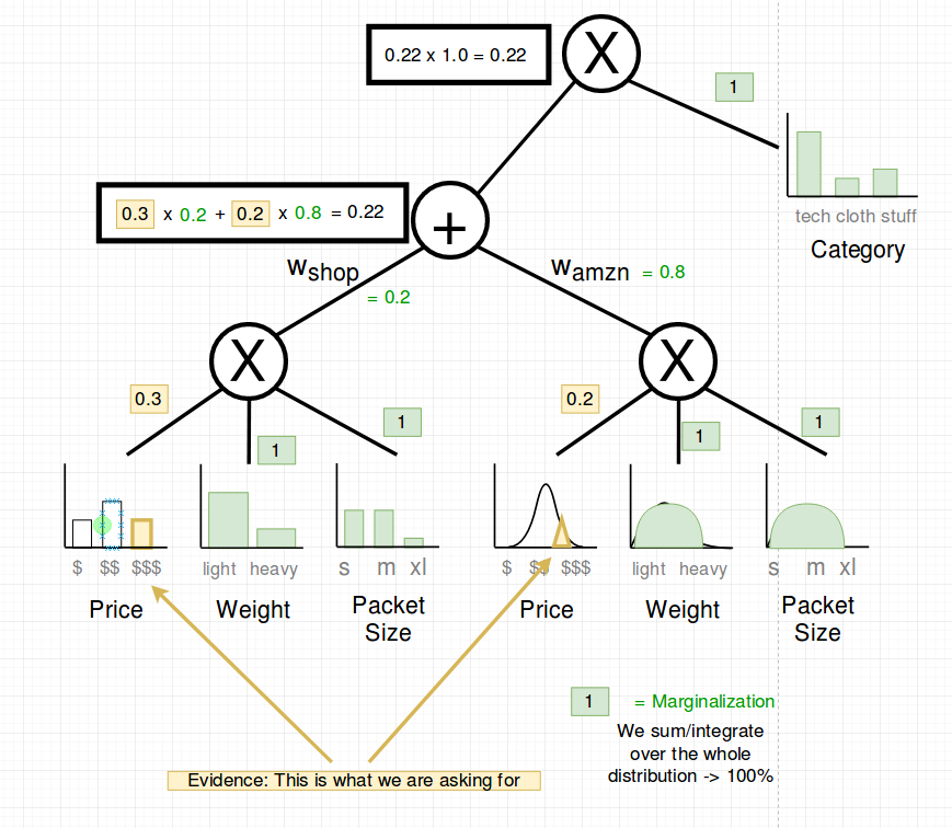
That’s it: Now we know that P(price=$$$) = 0.21

(Note: If the SPN is not normalized, then we would have to divide this result by the partition function Z)

All MAP States Are Computable in Linear Time

Let’s consider the case that it is sunday and we can only send light and small packages. What are the MAP states of the joint distribution?

In other terms: \(arg_{price, category} max P(Price=price, Category=category | Weight=light, Size=small)\)

How does it work?

1. We exchange the sum-nodes by max-nodes
2. Pick the mode or median of the random variables in question
3. Propagate upwards
4. Select subtree by following the max of the calculated weights under the max nodes

In the following picture you can see the max-node and the selected probabilities which are fixed (the evidence).

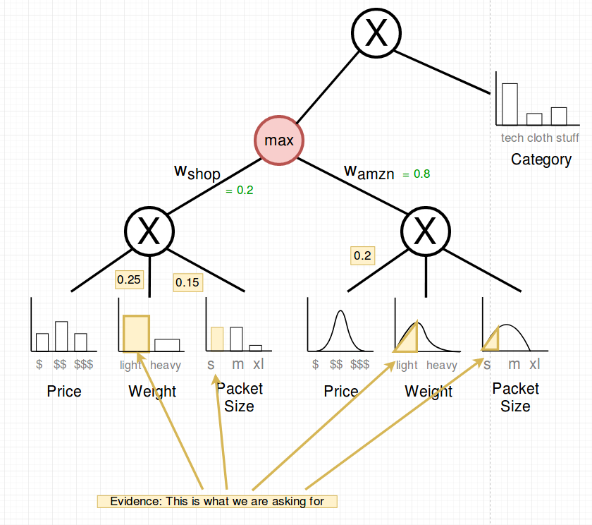
The median and mode are picked (in red). The following shows the upward pass:

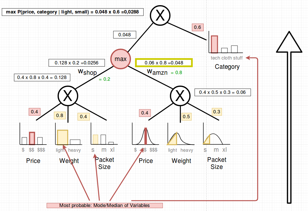
To select the maximum a-priori states we select the max paths when it comes to sums.

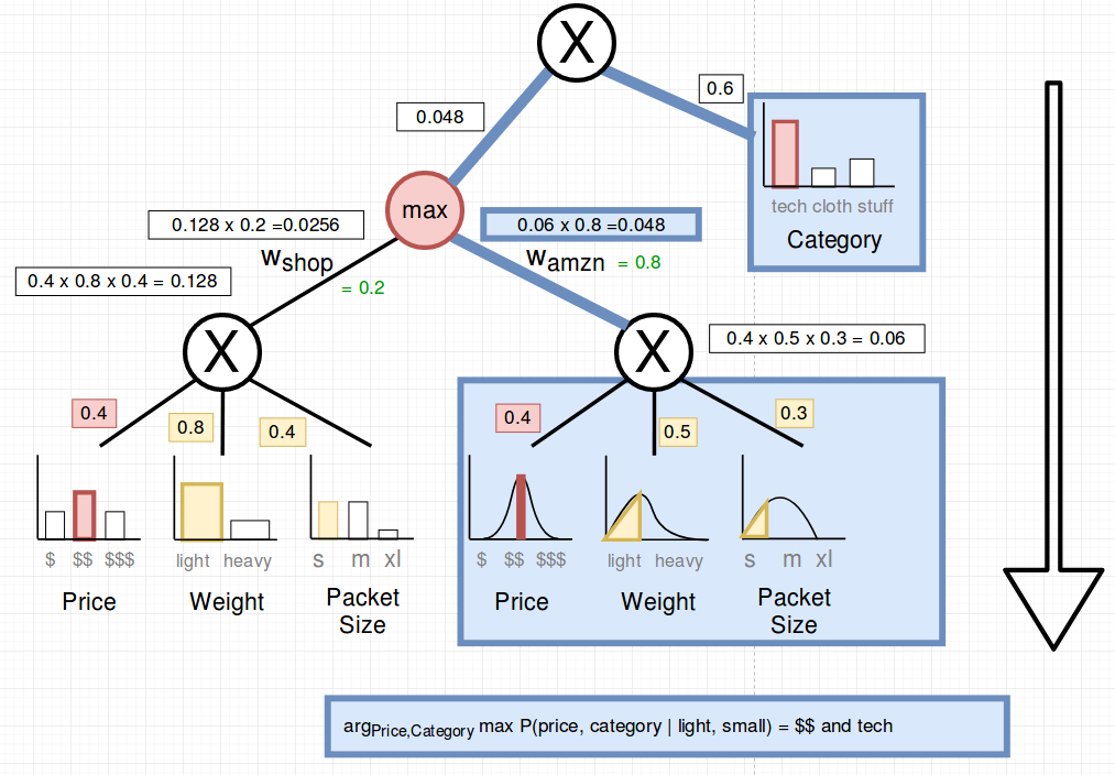
We found out that we should advertise medium priced tech if we only want to send small packets which are light.

What comes next?

In a subsequent post I am going to explain:

• how to learn the parameters of a SPN and
• how to learn the structure of an SPN.

Sources

https://www.youtube.com/watch?v=eF0APeEIJNw

http://spn.cs.washington.edu/talks/Gens_SLSPN_ICML2013.pdf

https://uwaterloo.ca/data-analytics/sites/ca.data-analytics/files/uploads/files/oct17spn-guest-lecture-stat946-oct17-2017.pdf