This article explains Hopfield networks, simulates one and contains the relation to the Ising model.

Hopfield Nets

Let’s assume you have a classification task for images where all images are known. The optimal solution would be to store all images and when you are given an image you compare all memory images to this one and get an exact match. But then you realize that this “look up” (comparing one image after another) becomes costly the more images you have to memorize. Even if you try to arange the images in a tree structure you will never be as fast as the following solution: store all images in Content addressable memory (CAM). CAM is specialized hardware that is used in routers. Ternary-CAM additionally has a “Don’t-Care” state (“?”) with which parts of the pattern can be masked (this is useful for IP routing).

In German CAMs are referred to as “Assoziativspeicher” (associative memory). Intuitively you don’t use an address to access data but instead you use data to access the address of the data.

Now imagine we had many pictures of dogs in our memorized array. And then comes a new image of a dog. Expect for the masking option (“?”) we cannot perform any kind of fuzzy search on hardware CAM.

As we will see in the following section, a Hopfield Network is a form of a recurrent artificial neural network and it serves as some kind of associative memory. It is interesting to analyse because we can model how neural networks store patterns.

Binary Hopfield Networks

A network with N binary units which are interconnected symmetrically (weight \(T_{ij}=T_{ji}\)) and without self-loops (\(T_{ii} = 0\)). Every unit can either be positive (“+1”) or negative (“-1”). Therefore we can describe the state of the network with a vector U. For example U = (+,-,-,-,+…).

Intuitively we initially set a state and wait until the network relaxes into another stable state. That means it does not change anymore once it reached that state. The reached state is the output value. For the associative memory example with images, the initial state is the image (black and white) and the stable state can also be interpreted as an image.

Each of the units is a McCulloch-Pitts neuron with a step-function as non-linearity. That means if we only update a single unit (“neuron”) then we calculate the weighted sum of the neighbours and set the neuron to “+” if the sum is greater or equals a threshold.

• Weighted sum of neuron \(x_j\): \(g(x_j) = \sum_{i}{x_i \cdot T_{ji}}\)
• Step function: \(x_j = \begin{cases} +1, g(x_j) \ge 0\\ -1, else \end{cases}\)

Update procedure:

• Synchronous update: A global clock tells all neurons at the same time to update. As a consequence all new states only depend on the old states
• Asynchronous update: One unit is updated after another. This seems to be more plausible for biological neurons or ferro-magnets because they have no common clock. The order is random.

Learning refers to finding appropriate weights. For the associative memory we want the connections between two neurons positive if they are often active together and we want the value to be negative if they are often different. This is Hebbian Learning Theory which is summed up as “Neurons that fire together, wire together. Neurons that fire out of sync, fail to link”.

Example

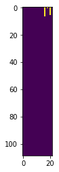
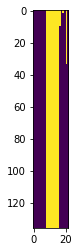
The following example simulates a Hopfield network for noise reduction. The training patterns are eight times “+”/”-“, six times “+”/”-“ and six times the result of “+”/”-“ AND “+”/”-“. The reason for the redundancy will be explained later.

The images of the simulations have the number of state at the x-axis and the time step as y-axis.

import numpy as np
import random
import matplotlib.pyplot as plt

patterns = [
#     Left variable                |    Right variable              =   Left AND Right    
    [-1, -1, -1, -1, -1, -1, -1, -1, -1, -1, -1, -1, -1, -1, -1, -1,   -1, -1, -1, -1, -1, -1],
    [-1, -1, -1, -1, -1, -1, -1, -1, +1, +1, +1, +1, +1, +1, +1, +1,   -1, -1, -1, -1, -1, -1],
    [+1, +1, +1, +1, +1, +1, +1, +1, -1, -1, -1, -1, -1, -1, -1, -1,   -1, -1, -1, -1, -1, -1],
    [+1, +1, +1, +1, +1, +1, +1, +1, +1, +1, +1, +1, +1, +1, +1, +1,   +1, +1, +1, +1, +1, +1]
]

size = len(patterns[0])
weights = np.array([[0]*size]*size)

for pattern in patterns:
    for i in range(0, size):
        for j in range(0, size):
            if j==i:
                pass
            else:
                weights[i,j] += pattern[i] * pattern[j]

def simulate(x1, x2, eps=30, first_state=None, visualize=True):
    number_of_iteration_unchanged = 0

    if not first_state:
        first_state = [x1]*8 + [x2]*8 + [+1, -1, +1, -1, +1, -1]
    trace = [
        first_state
    ]

    while (number_of_iteration_unchanged < eps):    
        if len(trace) > 1 and trace[-1] == trace[-2]:
            number_of_iteration_unchanged += 1
        else:
            number_of_iteration_unchanged = 0

        random_unit = random.randint(0, size-1)

        all_new_states = (np.array(np.dot(weights, trace[-1]) >= 0.0, dtype=np.int)*2) - 1
        trace.append(trace[-1].copy())
        trace[-1][random_unit] = all_new_states[random_unit].copy()

    np_trace = np.array(trace)

    if visualize:
        plt.imshow(np_trace)
        plt.show()

    return trace[-1]

simulate(-1,-1, eps=100);

simulate(1,1, eps=100)

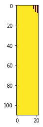
[1, 1, 1, 1, 1, 1, 1, 1, 1, 1, 1, 1, 1, 1, 1, 1, 1, 1, 1, 1, 1, 1]

simulate(-1,+1, eps=100);

simulate(+1,-1, eps=100);

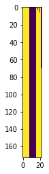
We see that all of the simulations “relaxed” to a solution which did not change for a long time (epsilon). Running the simulations multiple times showed that the (0,0) and (1,1) cases always converged to the correct pattern whereas the distinct cases were torn between the the correct state and its inverse.

But why does the network converge at all?

Stability theory

In system theory there is the quest to prove the stability of different kind of systems (see here). A system is said to be stable if small perturbations of the input data lead to small variations of the output value.

Stability can be intuitively grasped by imagining the velocity and phase of a pendulum. See the image by Krishnavedala.

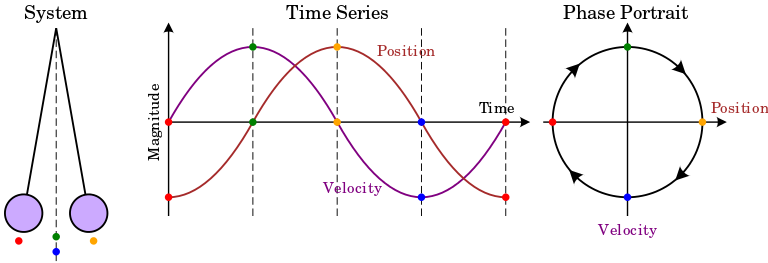
If the pendulum was damped the phase portrait would look like a spiral. The center to which it converges over time is a of point of attraction which is called equilibrium. The circle in the diagram is called “orbit”. An important question is for example: Will the trajectory of a given initial state converge to the point or will it diverge.

And what happens if the system gets “pushed” a little bit. A pendulum would oscilate a little bit and converge back to the equilibrium but a football on a hill would roll down.

For linear systems we can use the magnitude of the derivative of a point a. If it is less than one the system is said to be stable.

For more information see Stability theory on Wikipedia.

The Lyapunov Function can be used to show asymptotic stability (it gets really close) or lyapunov stability (all points which were at time t in an orbit are at t+1 in a small neighbourhood). It works by choosing a Lyapunov function which has an analogy to the potential function of classical dynamics. In real physical systems a precise Energy function can be used. You can imagine a state x of pendulum. If the system loses energy the system will reach a final resting point. The final state is the attractor. Lyapunov showed that it is not necessary to know the energy function but it is enough to find a Lyapunov function V(x) with the following criteria:

• \[V(0) = 0\]
• \(V(x) > 0\) if \(x \ne 0\)
• \(\dot{V}(x) = \frac{d}{dt}V(x) = \nabla V \cdot f(x) \le 0\) if \(x \ne 0\)

Lyapunov Stability

Energy function

Let’s apply this to Binary Hopfield Networks. We saw in the simulation that the Hopfield nets converge. Will this always be the case?

We choose our Energy function: \(E = -0.5 \sum_{j}{ \sum_{i \ne j}{u_i \cdot u_j \cdot T_{ji}} }\)

Actually we cannot assume to have a single global optimum on the surface of the energy function. At least every pattern we want to store should a local optimum. So we just show that the energy at t+1 is less or equal to t and therefore we always find a local optimum of the energy function.

In our asynchronous, random update procedure we pick a unit u. It either has the state -1 and we change it to +1 or it has the state +1 and we change it to -1. In the first case the difference is “+2” and the the second one it is “-2”. => \(\Delta u_j \in \{ -2, +2 \}\)

How does the energie of unit j change?

Define: \(\Delta u_j = u_{j_{new}} - u_j\)

Two possible cases for the neuron j:

“+2” case: The weighted neighbours are greater equal zero (\(\sum_{i \ne j}{u_{i} \cdot T_{ji} } >= 0\)), \(\Delta u_j=+2\), \(\Delta E_j = -1 \cdot (\sum_{i \ne j}{u_{i} \cdot T_{ji} }) \le 0\)

• “-2” case: The weighted neighbours are less than zero (\(\sum_{i \ne j}{u_{i} \cdot T_{ji} } < 0\)), \(\Delta u_j=-2\), \(\Delta E_j = +1 \cdot (\sum_{i \ne j}{u_{i} \cdot T_{ji} }) < 0\)

Conclusion: In both cases the energy either reduces or stays the same. Every minimum of the energy function is a stable state.

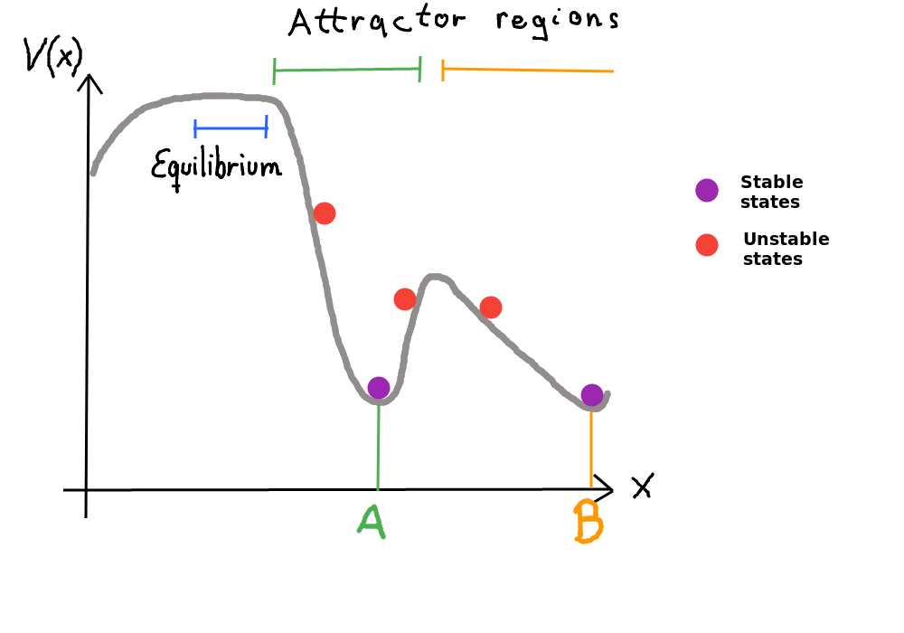
In the example of the associative memory we see that a pattern (state) can only converge to the correct solution (pattern) if it is in its attractor region. Imagine a 2d hill. On which side of the hill we roll down is determined by the random sampling process. This explains why the “AND-simulation” from above can converge into different states.

Note: Not all attractor regions have the same size. Therefore one state can attract more patterns than another. For the associative memory this leads to some kind of prior. Additionally mixture of an odd number of patterns cause mixture states which do not correspond to real patterns. Even numbers would sum up to zero.

For every pattern x the inverse of x is also a local minimum.

If we try to store too many patterns so called spin glass states are generated. They are no linear combination of the original states. A network of N units has the capacity to store ~ 0.15N uncorrelated patterns. All the minima that have no associated pattern are called spurious states.

If all weights are “+1” then the function calculated is something like k-Means/Hamming distance.

More math about Hopfield nets here.

Ising model

Hopfield nets are isomorph to the Ising model in statistical physics which is used to model magnetism at low temperatures. Every neuron equals an atom in a solid body. The state of the unit coincides with the spin (the magnetic moment). In the Heisenbergmodel the spin can be multivariate. In the Ising model the spin is either parallel or antiparallel to a given axis z). The latter can be written as the Binary Hopfield Network.

In physics the energy of the atoms is “measured” with the Hamilton operator H. It is the sum of the potential and kinetic energies in the system.

• \(s_i\) the spin of an atom
• \(T_{ij}\) the coupling constant between the spin of two atoms
• \(H\) is the strength of the magnetic field

The critical temperature was calculated with this model. A system with less than its critical temperature is dominated by quantum mechanical effects. If the majority of the couplings have a positive sign then the body is ferromagnetic. Which means you could use a permanent magnet to magnetize it like a refrigerator magnet.