This article tries to explain Boltzmann machines, RBMs, DBN, a little bit about energy models and contains a python example which shows how a generative model can be trained with contrastive divergence.

Boltzmann Machines

I have explained Binary Hopfield Networks in my last post. They had three main problems:

• Bad efficiency
• Spurious states
• No possibility of “escaping” the wrong attractor region

Hinton and Sejnowski worked with a probabilistic graphical model which they called Boltzmann machine (prev. Harmonium). The main differences:

• Every unit can have a unique bias
• The weighted sum that is calculated by each hidden unit has no threshold but a sigmoid activation function (the activation function is interpreted as the probability of the unit being active)
• Due to the stochasticity of the process a particle on the energy function can leave a local minimum

Generally speaking: A Boltzmann machine is a stochastic recurrent neural network with visible and hidden units. It is an undirected graph without self-connections.

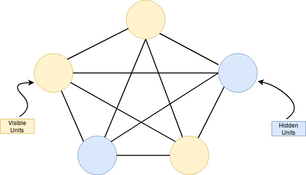
The structure of the net is generally not constrained and therefore sampling and learning become a big problem.

The hidden units are denoted with \(h_i\) and the visible units with \(v_i\). Both of these units are written as \(s_i\).

As mentioned above, every unit can either be active (1) or deactivated (0). Additional to the Hopfield Update rule we add a bias \(b_i\) and the sigmoid function:

\(z_i = b_i + \sum_{j}{s_j \cdot w_{ij}}\),       \(p(s_i=1) = \sigma(z_i) = \frac{1}{1+e^{-z_i}}\)

\(w_ij\) is the weight of the connection between i and j and vice versa (for i!=j).

Energy

Therefore we can write the energy of the network as:

This is different from the Hopfield Networks because of the bias. Although the weights are undirected, two connected units do not have to have the same bias.

What is the probability p(v) of a given state v? We defer the single probability of state to the energy function and divide it by all possible values of the Energy function:

(Z is the partition function)

Entropy and the Boltzmann distribution

If you measure the microscopic state of a thermodynamic system whose thermodynamic state is determined by a constant average energy, and only a constant average energy,

∑𝑖𝑝𝑖𝐸𝑖=⟨𝐸⟩

and you measure it many times, waiting between measurements long times in order to remove temporal correlations between them, then the set of measurements will follows the Boltzmann distribution

𝑝𝑖=𝑒−𝐸𝑖/𝑇∑𝑗𝑒−𝐸𝑗/𝑇

where 𝐸𝑖 is the energy of the i-th microscopic state, 𝑇 is the temperature and 𝑝𝑖

is the probability for each of the measurements to result in i-th microscopic state.

Notoriously, the Boltzmann distribution is the one you obtain if you maximize the entropy of the system

𝑆=−∑𝑖𝑝𝑖log2𝑝𝑖

as a function of the distribution 𝑝𝑖 subject to the set of thermodynamic constraints defining the thermodynamic state of the system, which in our case it is a constant average energy, only. This happens to be that way because, among all the microscopic states the system can possibly be, if you force the system to be in a specific thermodynamic state, then, you impose restrictions onto the set of microscopic states that the system can actually reach and with which probability (the 𝑝𝑖). This is the reason for which the thermodynamic state gives you some information about which are going to be your measurements about the microscopic states of the system. In other words, the entropy quantifies how much extra information you need, in average, to determine which is the microscopic state of the system at the time of your measurements, given that you only know its thermodynamic state.

source: quora

Heat

The more you know about the state of system, the more you can take advantage of it in order to extract energy from it. For example, if a rock is falling from the sky, you can extract energy from it if you know where it is going to fall. The more you know about how and where the rock is falling, the more energy you will be able to extract from the event. In a sort of analogy, knowing that a rock is falling from the sky is like knowing the macroscopic state. On the other hand, knowing where it is going to fall is like knowing the microscopic state.

Following the previous idea, you can only extract energy from a thermodynamic system from what you know of its microscopic state, which in the present context, it is the thermodynamic state. You can think of heat as energy contained in the system that you cannot extract from it because you ignore the precise microscopic state of the system at the moment where you want to extract the energy.

source: quora

Free energy

What is free energy? A thermodynamic quantity equivalent to the capacity of a system to do work.

The free-energy is then, in an average sense, the amount of energy contained in the system, i.e. it is total energy 𝑈=⟨𝐸⟩ minus the energy you cannot extract 𝑇𝑆 due to the remaining uncertainty or ignorance you have about which is its precise microscopic state the system is given that you only know about it its thermodynamic state.

This is free energy according to Helmholtz: Hemholtz free energy (U - TS)

There is also Gibbs free energy defined as

$ G = U + PV - TS = H - TS $

in which U is internal energy, P is pressure, V is volume, T is absolute temperature, S is entropy, and H is enthalpy.

It measures the usefulness or process-initiating work obtainable from a system at a constant temperature and pressure. If it is a chemical system, a reaction that lowers G occurs spontaneously.

source: quora

Where the sigmoid comes from

see wikipedia

The difference of energies of two states is

Substituting the energy of each state with its relative probability according to the Boltzmann factor (the property of a Boltzmann distribution that the energy of a state is proportional to the negative log probability of that state) gives:

where \(k_B\) is Boltzmann’s constant and is absorbed into the artificial notion of temperature \(T\). We then rearrange terms and consider that the probabilities of the unit being on and off must sum to one:

\(\frac{\Delta E_i}{T} = \ln(p_\text{i=on}) - \ln(p_\text{i=off})\) \(\frac{\Delta E_i}{T} = \ln(p_\text{i=on}) - \ln(1 - p_\text{i=on})\) \(\frac{\Delta E_i}{T} = \ln\left(\frac{p_\text{i=on}}{1 - p_\text{i=on}}\right)\) \(-\frac{\Delta E_i}{T} = \ln\left(\frac{1 - p_\text{i=on}}{p_\text{i=on}}\right)\) \(-\frac{\Delta E_i}{T} = \ln\left(\frac{1}{p_\text{i=on}} - 1\right)\) \(\exp\left(-\frac{\Delta E_i}{T}\right) = \frac{1}{p_\text{i=on}} - 1\)

Solving for \(p_\text{i=on}\), the probability that the \(i\)-th unit is on gives:

where \(T\) is referred to as the temperature of the system. This relation is the source of the logistic function found in probability expressions in variants of the Boltzmann machine.

Altering the factor T makes the logistic function wider or steeper.

Convergence

As with the Hopfield Nets the network shall converge to a stable state but “with a little bit of random”. This randomness is expressed by the steepness of the sigmoid function:

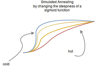
This steepness can be thought of as the learning rate of sgd. So we initially choose it large and then we let it become smaller so it can converge into a small region.

This is related to a method called simulated annealing. The size of the learning rate is called temperature and its getting colder with every step. The temperature determines the steepness in our example. The following image is taken from wikipedia to illustrate this process:

If the temperature is fixed and after enough unit updates the system only depends on the energy we say that it reached its thermal equilibrium.

Restricted Boltzmann Machines

In order to cope with some of the problems the model had to be restricted to a bipartite graph called the Restricted Boltzmann Machine. The two cores of the bipartite graph are the visible and the hidden units.

It was proven in 2010 by Long and Servedio that Z is intractable for both machines.

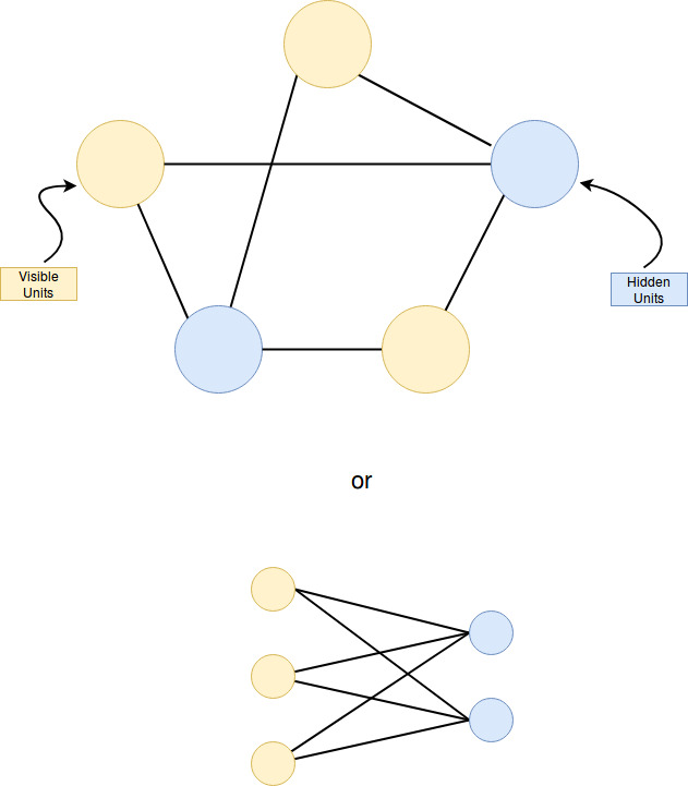
Energy

The probability of a visible unit v can be calculated easier:

And vice versa for a hidden unit:

The free energy in a RBM can be calculated and one might use it to tell something about the “potential energy” we still have when we converged to an equilibrium. It can be used to determine if a RBM is overfitting.

Learning with Contrastive Divergence

Source: Youtube

The idea is to pick a data vector and set it as visible units. Now because the graph is bipartite we can update all hidden units at the same time and vice versa with the visible units until the units of the RBM reached thermal equilibrium. This is a Markov Chain Monte Carlo method particularly Gibbs sampling.

The weight update becomes: \(\Delta w_{ij} = \epsilon ( <v_i h_j>^0 - <v_i h_j>^{\infty} )\)

This is a “fight” between what the memory wants (the state in the thermal equilibrium \(<v_i h_j>^{\infty}\)) and the data \(<v_i h_j>^0\). In the beginning the memory is random therefore we don’t want to make too many steps into its direction. If we don’t wait until the thermal equilibrium is reached but rather use the “wrong” gradient the method is called Contrastive divergence.

The longer the training continues the more iterations of contrastive divergence learning are used. In the beginning it is one and then we increase it.

Example of CD

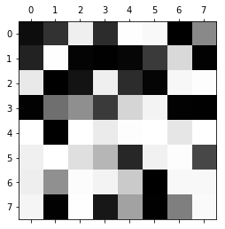
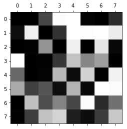
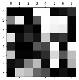
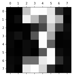
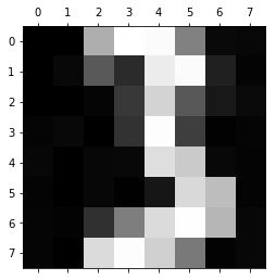
The following python snippet visualizes as training with CD on MNIST.

import matplotlib.pyplot as plt
import sklearn
import numpy as np

from scipy.stats import logistic
from sklearn.datasets import load_digits

digits = load_digits()

plt.gray()

<Figure size 432x288 with 0 Axes>

mask = digits.target == 3
threes = digits.images[mask]

# Init
h = np.random.normal(0, 1, 25)
# bias
b1 = np.random.normal(0, 1, 64)
b2 = np.random.normal(0, 1, 25)
# from x to h
W = np.random.normal(0, 1, [64, 25])

# parameter
lr = 0.01
iterations = 100
contrastive_divergence_steps = 50

# debug
print_every_nth = 100

# contrastive divergence CD-50

# train on the first 8 threes
for x in threes[:8]:
    for iteration in range(iterations):
        v = x.flatten() / np.max(x)

        p_of_h = logistic.cdf(W.T.dot(v) + b2)
        positive_phase = np.dot(v[:, np.newaxis], p_of_h[:, np.newaxis].T)

        for i in range(contrastive_divergence_steps):
            # plt.matshow(v.reshape([8,8]))

            # calculate p(h|v)
            p_of_h = logistic.cdf(W.T.dot(v) + b2)

            # sample p(h|v)
            h = p_of_h

            # calculate p(h|v)
            p_of_v = logistic.cdf(W.dot(h) + b1)

            # sample p(h|v)
            v = p_of_v

        if iteration % print_every_nth == 0:
            plt.matshow(v.reshape([8,8]))
            plt.show()
            print(iteration, " size of W: ", np.sqrt(np.sum(W**2)))

        negative_phase = np.dot(v[:, np.newaxis], p_of_h[:, np.newaxis].T)

        update = positive_phase - negative_phase

        W += lr * update

0  size of W:  39.924335666308195

0  size of W:  39.17467666748022

0  size of W:  38.97155882317313

0  size of W:  38.944982809345895

0  size of W:  38.80202589068636

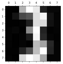
0  size of W:  38.74259814116064

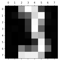
0  size of W:  38.6967212149249

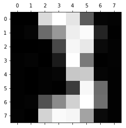
0  size of W:  38.74791680409241

This model of a three could already be used for dichotomizing threes and not-threes.

In the code I wrote something about a positive and a negative “phase” (or gradient). In the case of a correct sample the positive gradient increases the likelihood of the data whereas the negative gradient increases the likelihood of all others (which means that it decreases the likelihood of the current point).

There are discussions whether the latter might be something like “unlearning” what humans do when they dream.

Deep Belief Networks

Imagine we stacked another RBM on top of our hidden layer. We would treat the hidden units as visible and do the same training layer by layer (Greedy Layer-wise training). The RBMs are not really connected for the training. Once the first layer is ready we don’t train it anymore. This yields a Deep Belief Network which is something that Geoffrey Hinton has been working on for quite some time.

In contrast to the Hopfield Net and the Boltzmann Machine is a Belief Net a directed probabilistic graphical model. For this reason are the first models Markov Random Fields (MRF) and the Belief Net a Bayesian Net. The MRFs are coupled with Energy-based models because symmetric weights are an important property to converge. Directed graphs have the intention to model causal relationships and not only correlations.

The advantage of this “stacking” is to build hierarchical features. Although neural networks with two hidden layers are in theory already a general function approximator depth introduces a valuable inductive bias especially when coupled with a convolution. What I mean with that is that there are hierarchical patterns which can be uncovered easily when we assume locality and increasing complexity.

A Belief Net is:

• A directed acyclic graph
• typically sparsely connected (this is a prerequisite for some smart algorithms to work)
• every variable could be observed or hidden (“visible effects” and “hidden stochastic causes”)
• First target: Infer the state of unobserved variables
• Second target: “Learning”: Adapt the interactions between nodes in the graph in order to maximize the likelihood

Sampling the leaf nodes is easy but sampling the posterior is hard. Why is this interesting? In supervised learning we assume that all our training samples were sampled from the data manifold. Why can’t we just use the training data as samples from the posterior?

Unfortunately I have a technical answer only. For Variational Autoencoders (VAE). We assume that there are some hidden causes which we will never observe but we want to make them explicit and in the case of VAE even use them to control the generation of images or robotic hands.

An intuitively understandable reason for why sampling this posterior is difficult can be given by the concept of Explaining-Away. Explaining-Away is basically a pattern of reasoning where one cause of an effect explains that effect entirely thereby reducing (need not eliminate) the need to verify other alternative causes.

A quote from a quora answer:

Imagine an ‘observation’ ‘Ob’, say “you scored 100/100 in Math”. It could have had two (for the sake of simplicity) causes, viz ‘C1’ - ‘the question-paper was too easy’ and ‘C2’ - ‘you are too smart’. Now, ‘Ob’ could be because of either of those two causes (or both) i.e. you scored 100/100 because either the question-paper was way too easy or you’re just too smart or both. Confirmation of one cause, say ‘C1’ i.e. ‘paper was too easy’ doesn’t provide any evidence for the other alternate cause ‘C2’ (‘you are too smart’). But, in a probabilistic scheme of reasoning, confirmation of the first reasoning ‘C1’ (‘paper was easy’) SHOULD REDUCE the probability of the other cause (‘you are smart’) even though both can be true simultaneously. This is called “Explaining Away”. I mean to say if I know that you scored 100/100 and also know that the paper was way too easy, I tend to assume you’re not very very smart even if you actually are.

The variational approach that was kicked-off by the Wake-Sleep Algorithm just does not use an unbiased sample from the posterior but a more or less similar distribution. With this approximation we can make maximum likelihood. So it seems like we perform the same two steps as in Expectation Maximization.

There is a lot more to read and write about this topic but it feels like I am drifting to variational methods, therefore I am going end here and leave the rest for the next time.

A Practical Guide to Training Restricted Boltzmann Machines