In this post I am going to try to explain the basic concepts of localization of mobile agents which I have learned in the lecture “Lokalisierung mobiler Agenten” at the KIT.
The main outline:
- Wheel and vehicles (one lane kinematic model and differential model)
- Systems and discretization
- Euler method
- Dead reckoning
- Example: Error accumulating with constant velocity model
- Static localization (measurements, objective function and least squares)
- Angular measurements (atan2)
- Distance measurements (linearizing)
- Example: GPS
- Recursive Least Squares
- Bayesian Filtering Framework (Linear Gaussian Model)
- Dynamic localization (fusioning principles: BLUE, naive fusion, recursive fusion)
- Kalman Filter (derivation, optimality)
- Example: Tracking Car position and velocity
- Nonlinear Filtering (EKF, UKF, Particle Filter)
- EKF
- Wonham Filter
- Bingham Quaternion Filter
- SLAM
- Online SLAM (EKF-SLAM)
- Full SLAM (Graph-SLAM)
- Example: EKF-SLAM for 3d pose
- FAQ
Localization of Mobile Agents
Wheel and vehicles
As we don’t want to spend too much time on modeling forces and we assume that our mobile agents drive with moderate velocity on wheels we use the idealized wheel.
- It has a radius r, a wheel velocity \(\omega\),
- no slip in lateral direction
- no slip in longitudinal direction.
- It has point contact to the ground and
- only rolls into the direction of the steering angle
- it has no roll resistance.
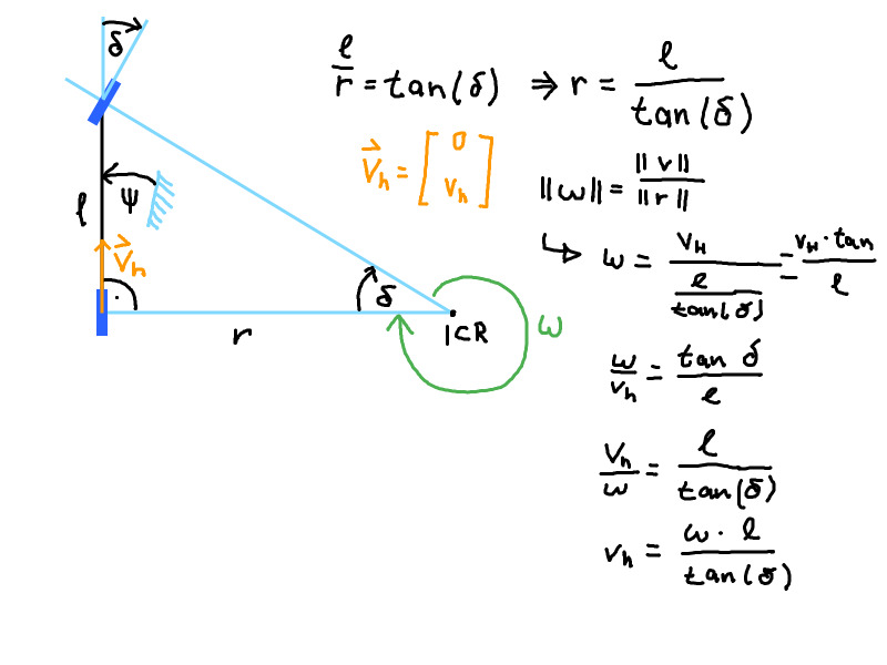
The Instantaneous Center of Rotation (ICR, “Momentanpool”) is the point where the wheel axis intersect. There are four different cases with our model:
- The axes meet at a point inside our outside of the vehicle and move on a circular path around the ICR.
- The wheel axes are on the same line. This is the case for the differential drive. The position of the ICR is controlled by the difference of the wheel velocities. If their difference is zero then ICR lays between the wheels.
- If wheel axes are parallel then the ICR is located at infinite distance. The vehicle is driving forward without a curved path.
- The wheel axes do not intersect at a single point. Within our model the vehicle is unable to move. Other models can handle this but they are a little bit more complex. For example: The dynamic one track model which models the slip angles of the wheels.
The magnitude form of the euler velocity equation (“Betragsform der eulerschen Geschwindigkeitsgleichung”) is used to set the angular velocity and the vehicle velocity into relation.
\[|\omega| = \frac{||v||}{||p||}\]where \(\omega\) is the angular velocity, v the vehicle velocity at a point at the vehicle and p the line from the ICR to the point.
For two different points p1 and p2 on the vehicle with different velocities v1 and v2, we can also use:
\[|\omega| = \frac{||v2 - v1 ||}{||p2 - p1||}\]Kinematic one track model
Differential drive
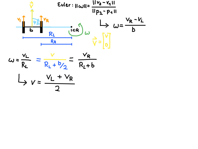
Note: If \(v_L + v_R = 0\) the ICR is at the center of the axis between the two wheels.
Systems
Let \(x\) be the state of the system, \(u\) the controllable inputs and \(w\) the uncontrollable changes to the state (like noise). The system equation \(a(x, \dot{x}, u, w) = 0\) holds. A simple specialization of this equation which we are going to use: \(\dot{x} = a(x, u, w)\)
If we manage to design \(a(...)\) in form a linear function then we can write our system in the following form and call it a Linear System:
\[\dot{x}(k) = A_k x(k) + B_k u(k) + w_k\] \[y(k) = C_k x(k) + D_k u(k)\]In the case that the system’s behavior does not change over time, we call it a Linear Time-invariant System (LTI):
\[\dot{x}(k) = A x(k) + B u(k) + w\] \[y(k) = C x(k) + D u(k)\]In order to access the state of the system at a point in time \(t\) we can use the the solution for the time-continuous linear time-invariant system:
\[x(t) = e^{A (t - t_0)} x_0 + \int_{t_0}^{t}{e^{A (t-\tau)} B u(\tau) d\tau }\]Discretization
Computers generally do not know how to solve time-continuous differential equations. The main problem is “how to solve the integral”? It is also difficult for humans if the antiderivative cannot be calculated.
For the use in digital computers we have to discretize the with respect to time, only then can we use it together with the discrete state sampling rate. So we introduce discrete timesteps \(t_k = k \cdot T_s, k \in \mathbf{Z}^+\).
Now we assume that the input signal is constant between two timesteps:
\[x(t_{k+1}) = e^{A T_s} x(t_k) + \int_{0}^{T_s}{e^{A (T_s - \tau)} B d\tau \cdot u(t_k) }\]Because the system is time-invariant we see that everything expect the x(t) and u(t) is constant, which leads us to the following discrete form:
\[x(t_{k+1}) = A' x(t_k) \cdot B' u(t_k)\]So we still have an integral here. How do we get A’ and B’?
With the use of the Laplace transformation if possible or numerical approximations.
Euler method
Given a differential equation which describes the system dynamics we want to calculate the state of the system after time t.
\[x(t) = x_0 + \int_0^t{\dot{x}(\tau) d\tau}\]We use the Euler Method. It tries to fit small rectangles under the curve of which we want to calculate the integral. If we use the height of the function at timestep \(t_k\) as the height of the rectangle we call it Forward/explicit euler. If the we use the height at \(x_{k+1}\) then it’s called Backward euler.
The backward euler is a little bit extra effort because you have to solve an equation to get to the next state but it has the advantage of being stable (solution can be found with the Newton method).
Instead of using the quotient of differentials we have to use the difference quotient.
\[\frac{d x(t)}{dt}\approx \frac{x(t + T_s) - x(t)}{T_s} = \frac{x_{k+1} - x_k}{T_s}\]In Matlab a continuous system can be transformed numerically with the command c2d:
sys_disc = c2d(sys_cont,Ts)
Until rounding errors happen in the computer, a smaller \(T_s\) leads to a better approximation.
Solution 3
Constant acceleration or constant velocity models.
Dead reckoning
Definition:
The task of dead reckoning is to get the pose of an object with respect to an external coordinate system.
To solve this task formulate a motion model in the object’s coordinate system.
Advantages:
- High sampling rate
- No infrastructure needed
- low latency
Disadvantages:
- Pose is only relative
- Accumulated error which leads to drift
How it works: We measure increments from the last state (change of place, velocity or acceleration). And then we use this measured information as system input to our discrete system model in order to calculate where our current position should be next.
“Schritthaltend”: Abtastrate höher als Rechenzeit für neuen Zustand.
Error
The total error of a linear system depends on all noise vectors:
\[e_k = x_k - x_{k}^{\text{ground truth}} = e_k (w_{k-1}, ..., w_0)\]For linear systems: The longer ago the error has been added, the more influence it has, because the exponentiated system matrix usually becomes larger over time:
\[e_k = A^{k-1}\cdot w_0 + A^{k-2}\cdot w_1 + ... + A\cdot w_{k-1}\]Important Note: When talking about the error it is important to realize that the error is not the difference between the estimate and the measurement but it is the difference between the ground truth and the estimate!
(The ground truth could be manually annotated or retrieved with another system, for example with a VICON or GPS)
Static localization
Sensors measure absolute pose in world coordinates.
Advantage
- No increasing error (“keine Fehlerfortpflanzung”)
Disadvantage
- External infrastructure necessary
Measurement principles
- Time-of-Flight
- Radar
- visual (cameras)
- strength of a signal (WLAN, Bluetooth, GSM)
The measurement function z = h(x) generates a measurement from the true pose of the robot.
\[z \in R^M , x \in R^N, M >= N\]Example 1: Trilateration
You want to localize the robot by measuring the distance to point landmarks.

The ith measurement is the distance to the point i (with coordinates p_x and p_y). The robot’s position is x_x, x_y.
\[z_i = \sqrt{ (x_x - p_x)^2 + (x_y - p_y)^2 } = || p - x ||\]ToDo: Linearize!
The vector z contains the measurements to all the landmarks: \(z = [z_1, ..., z_M]^T\) And we assume that the measurement function h(x) produced this vector \(z = [h_1(x), ..., h_M(x)]\).
This leads us to a non-linear least squares (LSQ) problem with the objective function and the weighting matrix W (pos. definite):
\[arg_x min G(x) = ||z - h(x)||^2_W = (z - h(x))^T W^{-1} (z - h(x))\]The weighting matrix allows us to express our knowledge about the measurements. Whether we want to trust the measurement of one sensor more than others.
Once we solve this optimization problem we will localize the robot. If we cannot write the measurement function as a linear equation then we could do this numerically.
If we can write the function as a linear equation then we can solve the problem analytically by deriving it, setting the derivation to zero and solving for x. (If we do not knew the orientation of the parabola then we would also have to check whether the optimum is a minimum or a maximum by checking the sign of the second derivation).
Example 2: Trilateration with walls
Let’s go back to the example and see whether we can reformulate the measurement function. Let’s assume that the landmarks are points on walls of a room.
In this case we can model the walls with Hesse’sche Normalform \(n_i * x + d_i = 0\) with \(||n_i||^2 = 1\) and \(d_i\) the distance to the wall.
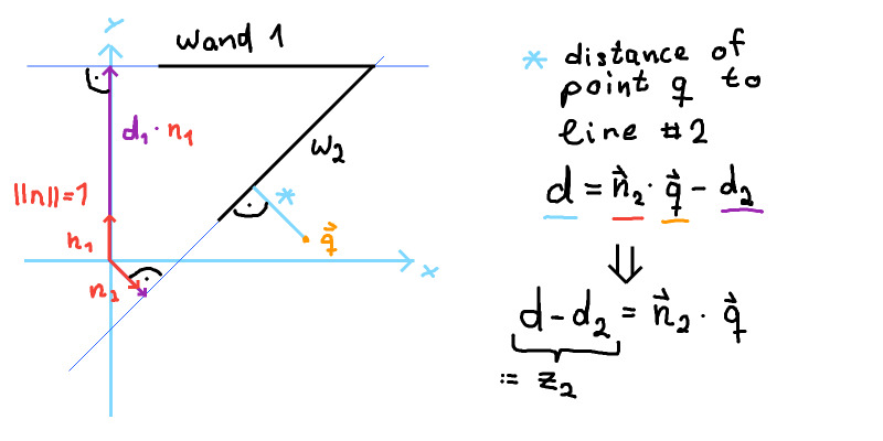
The distance to the ith wall is \(s_i(x) = h_i * x + d_i\)
\[s_i(x) - d_i = h_i * x\] \[z_i = h_i * x\] \[z_i = [h_{i_x}, h_{i_y}] * [x y]^T\]Which is a linear equation.
In the easiest case where we have exactly as many observations as state variables we obtain a quadratic measurement matrix:
\[[z_0, z_1] = [h_{0_x}, h_{0_y}; h_{1_x}, h_{1_y}] * [x y]^T\] \[z = H x\]=> \(x = H^{-1} z\)
We see that it would be convenient to always use a quadratic measurement matrix H but it has the downside that we would not use all of our measurements if we have more walls in the room and therefore we would be more error prone if one of the sensors returns a noisy value.
Least Squares
That’s why we come back to the LSQ which minimizes the sum of the squared errors between our measurements and the estimated state.
\[arg_x min G(x) = ||z - H x||^2_W = (z - Hx)^T W^{-1} (z - Hx)\]Multiplying the terms:
\[G(x) = (z - Hx)^T W^{-1} (z - Hx) = z\] \[z^T W^{-1} z - x^T H^T W^{-1} z - z^T W^{-1}Hx + x^T H^T W^{-1} H x\]Derive:
\[\frac{d }{d x} G(x) = - H^T W^{-1} z - z^T W^{-1}H + 2 H^T W^{-1} H x\]Set to zero:
\[-2 H^T W^{-1} z + 2 H^T W^{-1} H x = 0\] \[+ 2 H^T W^{-1} H x = +2 H^T W^{-1} z\] \[H^T W^{-1} H x = H^T W^{-1} z\] \[x = (H^T W^{-1} H)^{-1} H^T W^{-1} z\]Checking the second derivative:
\[\frac{d }{d x} -2 H^T W^{-1} z + 2 H^T W^{-1} H x z\] \[2 H^T W^{-1} H z\]Check whether it is positive definite:
\[2 H^T W^{-1} H z > 0\]Important: H has to have at least full column rank otherwise the first bracket could not be inverted. This means that the columns have to be linearly independent of each others. Full column rank is the same as saying that rank(H) = dim(x) which enough to make rank(H) >= dim(x) true.
Note: If the weight matrix W is only semi-definite then the matrix \((H^T W^{-1} H)\) then the inversion is not uniquely determined (infinite solutions). We can still choose one by picking the with the smallest norm ||x||^2.
How to choose W? Diagonal matrix, positive definite. A large entry on the diagonal like 999 becomes 1/999 after inverting the matrix. And the multiplication with such a small value nearly cancels its influence onto \(\hat{x}\). Therefore: Large values in W result in mistrust for the related sensor value.
Example 3: Triangulation
If we can’t measure the distance to known landmark there might be the possibility to measure the angle.
The measurement equation:
\[\alpha_i = atan2(y_{LM}^i - y, x_{LM}^i - x) - \psi\]is not linear.
A quick reminder. The tan(x) looks like this:
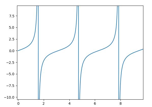
Which is undefined at 90 degree because it is sin(90) / cos(90) and cos(90) is zero.
The atan2 is defined as the angle between the x axis in the range between ]-pi, pi]:
It resolves the ambiguity that -90 degree is the same as 270 degree.
Recursive Least Squares
The normal least squares method has the downside of processing all measurements in one matrix. In reality the measurements are obtained incrementally and we do not want to repeat the processing of the measurement matrix again and again. Especially when it is becoming larger and larger.
The recursive least squares fusions the last result with the newly obtained measurement. The measurement matrix’s size stays constant and therefore the processing time.
We are now going to work with batch matrices. They are matrices whose entries are matrices themselves.
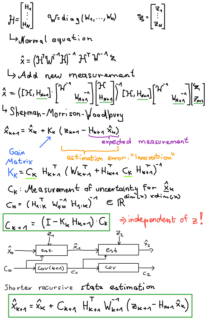
It is important that the block weight matrix W is a diagonal matrix. If that is not the case then we have to diagonalize it: \(W = V^T D V\).
Note: \(C_k\) can be calculated independently if H and W are independent of the measurements. With this in mind we see that with \(k to \infty: C_k\) ~= 0
We obtain recursive equations which we can solve for every timestep in constant time. But how do we start the recursion?
There are two options:
- Wait until we have N measurements where N = dim(x). Then H is quadratic so we easily invert it directly. And we calculate \(C_k = (H_{1:K}^T W_{1:K}^{-1} H_{1:K})^{-1}\)
- We initialize x with the zero vector and set its uncertainty to infinite by defining \(C_k = \lambda \cdot I\) where I is the identity matrix and \(\lambda\) a large positive number.
Information form
With the relationship: \((I - K_k H_{k+1}) = C_{k+1} C_{k}^{-1}\)
we can transform the prediction:
\[x_{k+1} = (I - K_k H_{k+1}) x_k + K_k z_{k+1}\]… to:
\[x_{k+1} = C_{k+1} C_k^{-1} x_k + C_{k+1} H_{k+1}^T W_{k+1}^{-1} z_{k+1}\]Wikipedia states: In the information filter, or inverse covariance filter, the estimated covariance and estimated state are replaced by the information matrix Y and information vector y respectively.
We multiply \(C_{k+1}^{-1}\) on both sides left:
\[C_{k+1}^{-1} x_{k+1} = C_k^{-1} x_k + H_{k+1}^T W_{k+1}^{-1} z_{k+1}\] \[y_{k+1} = y_{k} + H_{k+1}^T W_{k+1}^{-1} z_{k+1}\]And the Inverse Covariance matrix is calculated like this:
\[C_{k+1}^{-1} = C_{k} + H_{k+1}^T W_{k+1}^{-1} H_{k+1}\] \[Y_{k+1} = Y_{k} + H_{k+1}^T W_{k+1}^{-1} H_{k+1}\]But why?
- In this inverse formulation of the covariance matrix we can define infinite mistrust with a simple zero
- As long as we do not need any steps in between, we can calculate the information matrix and information vector separated from each others
- Biggest advantage according to Wikipedia: “The main advantage of the information filter is that N measurements can be filtered at each timestep simply by summing their information matrices and vectors.” (“Kovarianz wird additiv”)
Bayesian Filtering Framework
We are going to approach the localization from a probabilistic context. We treat the state \(x\) as a probability density function over the state space with its expectation value as the most likely position and the covariance matrix of the pdf as the measure of uncertainty.
This is equivalent to hidden markov models.
Estimate the current state after all the measurements of the past:
\[P(x_k|z_{1:k}) =^{\text{Bayes}}= \frac{P(z_k|x_k, z_{1:k-1}) \cdot P(x_k|z_{1:k-1})}{P(z_k|z_{1:k-1})}\]With the Markov assumption:
\[\frac{P(z_k|x_k) \cdot P(x_k|z_{1:k-1})}{P(z_k|z_{1:k-1})}\]The partition function might not be tractable therefore we continue with a term which is proportional to the last one:
\[P(z_k|x_k) \cdot P(x_k|z_{1:k-1})\]\(P(z_k\|x_k)\) is a probabilistic form of the observation model.
The probability of a state given the past observations is the prediction problem: \(P(x_k|z_{1:k-1}) = P(x_{k+1}|z_{1:k})\)
We can marginalize this: \(P(x_{k+1}|z_{1:k}) = \int_{x_k}{P(x_{k+1}|x_k, z_{1:k}) \cdot P(x_{k}|z_{1:k})}\)
If we assume time invariance then we can write:
\[P(x_{k+1}|z_{1:k}) = \int_{x_k}{P(x_{k+1}|x_k) \cdot P(x_{k}|z_{1:k})} dx_k\]\(P(x_{k+1}\|x_k)\) is the probabilistic version of the system model.
And \(P(x_{k}\|z_{1:k})\) is the question where we started but one timestep earlier. So we see that we can solve this problem with recursion.
The main problem with this is the integral after the marginalization. A restriction is necessary to solve it.
Linear Gaussian Model
“A linear-Gaussian model is a Bayes net where all the variables are Gaussian, and each variable’s mean is linear in the values of its parents. They are widely used because they support efficient inference. Linear dynamical systems are an important special case. “ - metacedemy
\[x_{k+1} = A_k x(k) + B_k u(k) + w_k\] \[z_k = H_k x(k) + v_k\]Where:
- \(A_k\) is the system model
- \(B_k\) the input matrix
- u(k) the controllable input vector
- \(w_k\) the normally distributed white process noise (-> mean=0, cov=\(C_w\))
- \(H_k\) the measurement matrix
- \(v_k\) the normally distributed white measurement noise (cov=\(C_v\))
As a result: x(k) and z(k) are also random variables with \(N(\hat{x}, C_x)\) and measurement uncertainty \(C_z\).
Summary: The state and the measurement are random variables. The Bayesian Framework is helpful to see how a filter should calculate the posterior distribution from the prior distribution, measurements, the measurement model and the system model. The mentioned restriction of the motion model leads to the fact that we have only one possible predecessor for a given state. As a result, we do not have to build the integral in the Bayesian Framework anymore.
Filter Step without priori knowledge
“Filterschritt ohne Vorwissen”
We start with the measurement equation of the linear system.
\[z_k = H_k x_k + v_k\]Attention: dim(z_k) >= dim(x_k) and H full column rank.
A first non-formal way is to use the deterministic Least Squares for the random variable mapping with the unknown weight matrix W:
\[x_k^{LS} = (H_k^T W_k^{-1} H_k)^{-1} H_k^T W_k^{-1} z_k\]And then determine the first and second moment:
Expectation value: \(\hat{x}_k^{LS} = (H_k^T W_k^{-1} H_k)^{-1} H_k^T W_k^{-1} \hat{z}_k\)
Covariance matrix: \(C_k^{LS} = (H_k^T W_k^{-1} H_k)^{-1} H_k^T W_k^{-1} C_k^z W_k^{-1} H_k (H_k^T W_k^{-1} H_k)^{-1}\)
This solution contains the unknown weighting matrix and has no proof of optimality in any way.
Therefore the next step is to derive a better solution with formal restrictions:
- Affine estimator (“linear”)
- Unbiased
- Minimum covariance (“best”)
These requirements form the “Best Linear Unbiased Estimator” (BLUE)
We start with an affine estimator:
\[x^e_k = K_k z_k + c_k\]We require (2) that the expectation value of the estimator is the same as of the real value (which is unknown) \(E[x^e_k] = E[x_k]\)
\[E[x^e] = K_k E[z_k] + c_k\]Now we use the measurement model:
\[E[x^e] = K_k H_k E[x_k] + c_k\]\(c_k\) has to be zero in order to let the estimator be unbiased:
\[E[x^e] = K_k H_k E[x_k]\]Now we add that the expectation values should be the same:
\[K_k H_k E[x_k] = I E[x_k]\]This brings us to the following relationship which is not unique.
\[K_k H_k = I\]This is where our third requirement comes into play: We want the Cov(x_k^e)=C_k^e to be minimal. We can formulate this demand with the inverted observation model and the least squares approach:
\[x_k^e = K_k^{opt} z_k\]with
\[K_k^opt = (H_k^T (C_k^z)^{-1} H_k)^{-1} H_k^T (C_k^z)^{-1}\]We calculate the covariance matrix like this:
\[C_k^e = (H_k^T (C_k^z)^{-1} H_k)^{-1}\]Note: We get the same result for the formal approach and the initial least squares solution if we use the covariance matrix of the measurement as our weighting matrix.
Optimal fusion
Now we have the case that there are two unbiased but uncertain state estimations \(x_1\) with covariance \(C_1\) and \(x_2\) with \(C_2\).
- Linear estimator
- Unbiased
\(x_1\) and \(x_2\) are unbiased.
\[= K_1 E[x] + K_2 E[x]\] \[(K_1 + K_2) \cdot E[x] =^{!}= E[x]\] \[K_1 + K_2 = I\]We can reduce the amount of work by only defining one weighting matrix K and its opposite:
\[K = K_1\] \[K_2 = I - K\]And plug it into the estimator:
\[x^e = K x_1 + (I - K) x_2\]The covariance matrix of the estimator becomes:
\[C^e(K) = K^T C_1 K + (I - K)^T C_2 (I - K)\]As with the filter step without bias, we want the uncertainty of the combination to be minimal. We achieve this by projecting the covariance matrix onto a unit vector, deriving this projection, setting the derivate to zero and then solve for the optimal K.
Projection: \(P(K) = e^T C^e(K) e\)
Derivative:
\[\frac{d}{dK} P(K) = 2 e e^T (K C_1 + (I - K) C_2)\]Set to zero:
\[2 e e^T (K C_1 + (I - K) C_2) = 0\] \[K C_1 - (I - K) C_2 = 0\] \[K C_1 - C2 + K C_2 = 0\] \[K C_1 + K C_2 = C_2\] \[K (C_1 + C_2) = C_2\] \[K = C_2 (C_1 - C_2)^{-1}\]Finally the optimal fusion of two unbiased states:
\[x^e = C_2 (C_1 + C_2)^{-1} x_1 + C_1 (C_1 + C_2)^{-1} x_2\]With the new Cov:
\[C^e = C_2 (C_1 + C_2)^{-1} C_1\]Prediction
First of all we rewrite our linear model a little bit. We assume that the input random vector is a sum of a known input vector \(\hat{u}_k\) and process noise \(w_k\).
\[x_{k+1} = A_k x_k + B_k (\hat{u}_k + w_k)\]The expectation value of the prediction becomes:
\[x_{k+1}^p = A_k \hat{x}_k + B_k \hat{u}_k\]Under the assumption that the system noise is not correlated to the old state we obtain the new covariance matrix:
\[C_{k+1}^p = A_k C_k^x A_k^T + B_k C_k^w B_k^T\]Dynamic Localization
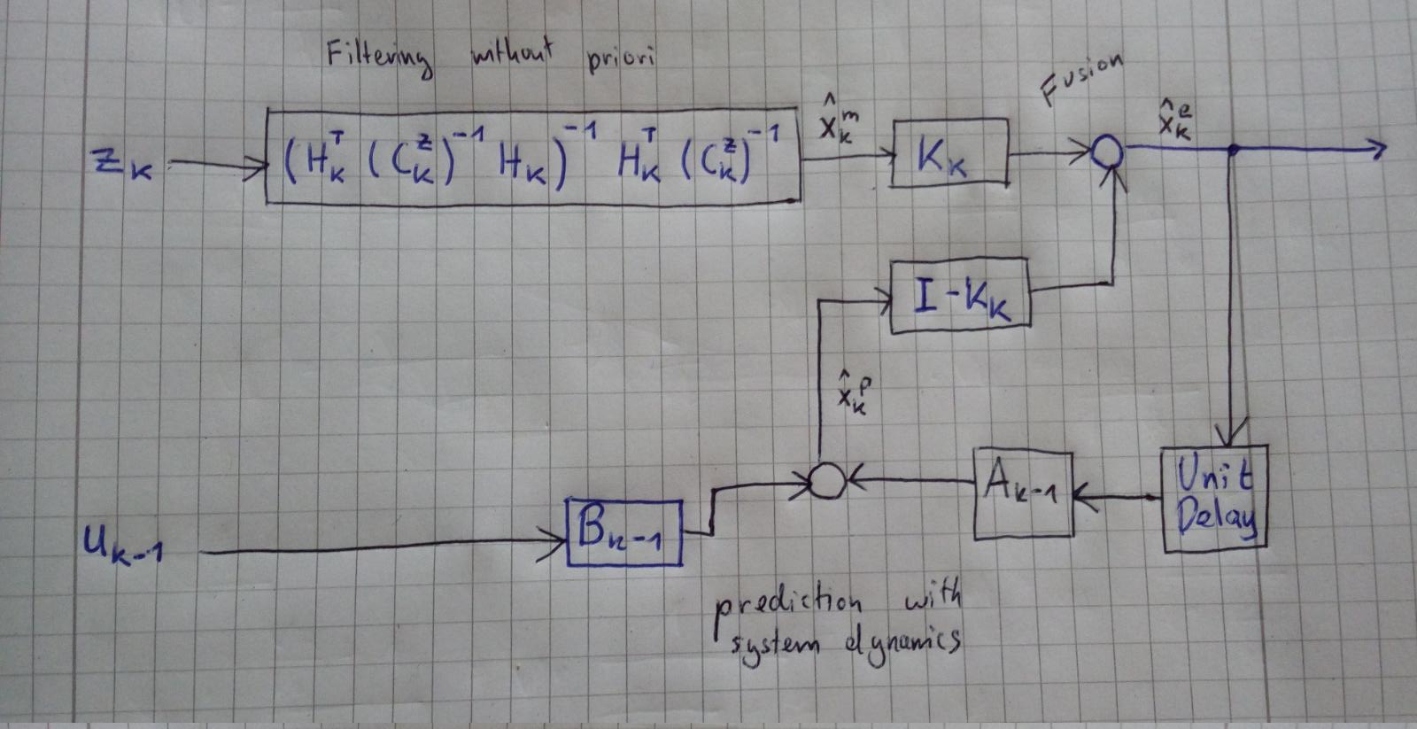
Use the optimal fusion, dead reckoning and prediction to build the naive recursive estimator.
Important: Because we are going to calculate a full state from the given measurement we have to require the \(dim(z_k) >= dim(x_k)\)
It works as follows:
- Get a measurement z
- Deduce a state variable from z and C_z
- Use the system dynamics to predict the state variable until we have a new measurement
- Deduce a new state from the new measurement
- Use a BLUE estimator which fusions the predicted state and the deduced state from the new measurement
Kalman filter step
In the Kalman filter step we assume that the dimension of the measurement vector is smaller than the dimension of the state vector and we have priori knowledge.
When a new measurement arrives, the predicted state and the measurement matrix are used to “generate” a predicted measurement that gets compared to the true measurement. The difference between both is called the innovation and it is used to correct the predicted state.
We are looking for a BLUE estimator again:
Linear estimator:
\[x^e = K_1 x^p + K_2 z_k\]shall be unbiased (the predicted estimation and the z_k are also unbiased):
\[E[x^e] = K_1 E[x^p] + K_2 E[z_k]\] \[E[x] = K_1 E[x] + K_2 H_k E[x]\] \[I = K_1 + K_2 H_k\] \[K = K_1\] \[K_2 = I - K H_k\]Third requirement: Minimum variance. Again with projection onto a unit vector and minimizing we get:
\[C_k^e = (I - K_k H_k) C_k^p\]A popular interpretation of the Kalman filter step uses a different formulation of the filter:
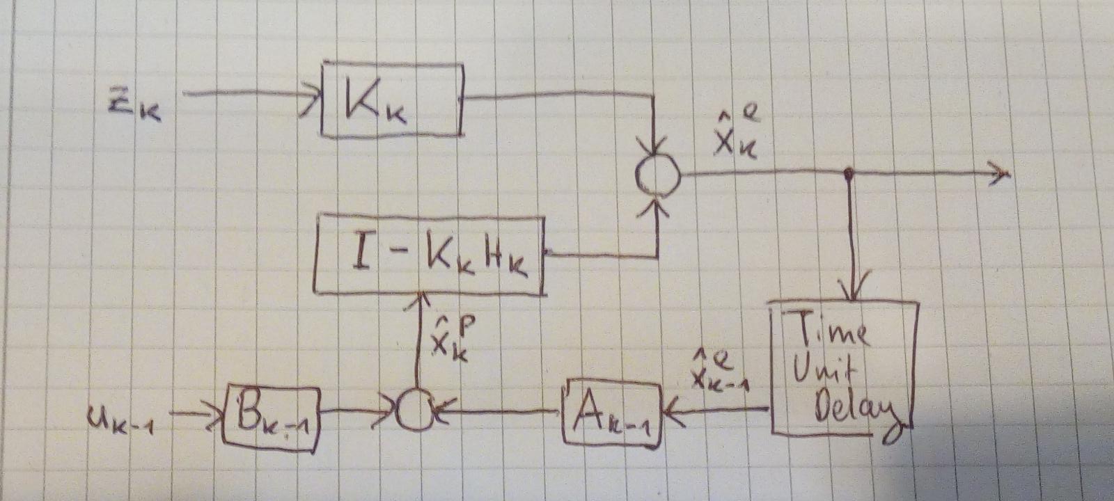
\[\hat{x}_k^e = \hat{x}_k^p + K_k (z - H_k \hat{x}_k^p)\]The difference in the brackets is called “innovation”. And the difference is multiplied by the Kalman Gain Matrix. In block diagrams this can be written as a controller (more specific a “regulator”) that regulates the difference between the measurement and the projected measurement to zero with a proportional factor of K.
Recursive Kalman estimator
The recursive Kalman estimator works the same as the recursive estimator but it uses the Kalman filter step. This means that a new measurement is not transferred into state space instead it gets compared directly to a predicted measurement of the predicted state. The difference is multiplied by the Kalman gain and added to the predicted to state. This way the Kalman filter only stores the mean and covariance of the state estimation and it also does not get more complex with the number of used measurements.
Approximation of general systems
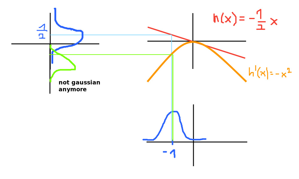
When we are dealing with a nonlinear system and we can’t trick it into linearity then we have to linearize it.
If we don’t do this, then the main problem becomes that we are not mapping from gaussian to gaussian. The following image shows the blue gaussian curve projected by a linear function h(x) and by a nonlinear function h’(x).
We solve this by linearizing the system model \(x_{k+1} = a(x, u)\) and the measurement model \(z = h(x, v)\). Why? Because all of our equations until now only work with matrices A, B and H.
The first order Taylor polynomial is used:
\[x_{k+1} = a(x, u) \approx a(x, u) + J_{a, x}^x \cdot \Delta x + J_{a, x}^u \cdot \Delta u\]\(J_{a, x}^u\) is the jacobi matrix of function \(a\) around the point \(x\) containing the partial derivatives only after u.
\[x_{k+1} \approx a(x, u) + J_{A_k} * \Delta x + J_{B_k} * \Delta u\]This is a linear equation but it still does not look like the system equation that we need for our Kalman filter.
But if we stop modelling the full state of the system and only track the difference between the states (\(x_{k+1} \approx x_{k} + \Delta_{x_k}\)) we get the form in which we are interested:
\[\Delta x_{k+1} \approx J_{A_k} * \Delta x_k + J_{B_k} * \Delta u_k\]Note: If the system was time invariant or the development point around which we linearized was an equilibrium point, the Jacobi matrices are also time invariant.
We linearize the measurement model in the same way:
\[\Delta z_k \approx J_{H_k} * \Delta x_k\]The Extended Kalman Filter (EKF) is the regular Kalman filter using these linearized equations.
The predicted state is the linearization point.
???
ToDo: Mitschrieb Vorlesung 12
???
UKF
The problem with EKF is that large uncertainties or large \(\Delta\)s are not transformed correctly when the nonlinear function is only linearized at one place.
Therefore the Unscented Kalman Filter uses so called sigma points to represent remarkable points of the input normal distribution, transforms them with the nonlinear function and reestimates a new normal distribution from the new sigma points.
Particle Filter
The procedure of the UKF is already close to the Particle filter. Here we represent the priori distribution with particles instead of a parametric function. Then the particles are transformed by the nonlinear function. The function might not be deterministic, it could add random noise.
The predicted particles are weighted according to a distance measure of a new measurement. For example: Particles which are close to the real measurement get a large weighting.
In order to avoid degeneration of the particles we resample the particles by sampling the same number of particles but not uniformly. The distribution from which we sample is the distribution of the samples.
As a result we obtain many particles near the location where a single particle with large weight had been. And random other particles.
The particle filter is also called Sequential Monte Carlo.
SLAM
Simultaneous Localization and Mapping is a “Chicken and Egg” problem. We don’t know the pose of the robot and neither the positions of the landmarks but we want to create a map and localize the robot within.
Challenges:
- Nonlinearities
- Data association: which measurement belongs to which landmark
- Complexity of big maps
- Non-static environment
Approaches for 2d SLAM:
- Online SLAM -> Map and last pose. The state contains the last pose and the landmarks: \(x^T = [x,y,\phi, LM_1^x, LM_^y, ..., LM_L^x, LM_L^y]\). It has a size of 3 + 2L. The Covariance matrix has the size squared entries.
- Full SLAM -> Map and trajectory The state contains 3k + 2L entries.
EKF SLAM
Initialization:
- Naive init: Estimate the number of landmarks the robot is going to see and initialize the values with zero and infinite uncertainty
- Preferred init: Start with a small state vector and expand it every time a new landmark has been measured.
Whether it is a new landmark or a measurement belongs to an already known landmark is called the data association problem and an easy approach is to use 1-Nearest-Neighbour with the Mahalanobis distance that gets weighted according to the uncertainty of the landmarks. If this distance is above a threshold we see a new landmark.
Prediction:
The landmarks are static accordingly they do not move and no change in position has to be predicted. The robots moves as usual. The dead reckoning then adds uncertainty to the robot pose and consequently we also have to increase the uncertainty between the landmarks and the robot’s pose but the uncertainty between landmarks is not updated.
Attention: For the prediction of the mean we just apply the nonlinear motion model to the robot’s pose: \(x_{k+1}^p = a(x_k^e, u_k)\). For the prediction of the covariance matrix we do have to linearize \(a(.)\) with the Jacobi matrix J_{A_k}.
\[C_{k+1}^p = J_{A_k}^T C_k^e J_{A_k} + C_k^w\]\(C_k^w\) is an all zeros matrix except for the robots covariance which gets an additive noise term due to the system noise.
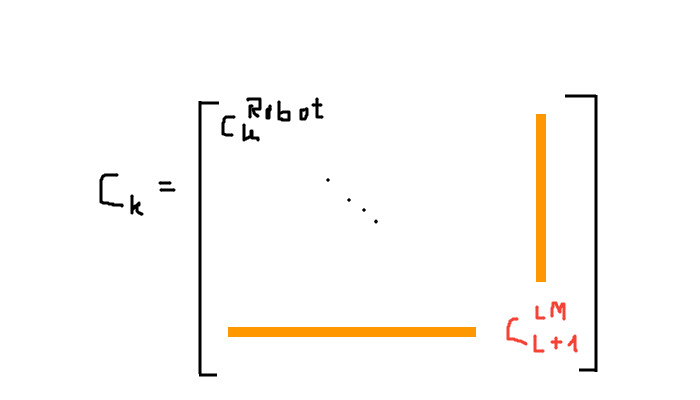
Only the first column and first row are updated by the prediction step:
\[C_{k+1}^p = \begin{bmatrix} C_{k+1}^{Robot} & C_{k+1, 1}^{Robot,LM} & \dots & \dots & C_{k+1, L}^{Robot,LM} \\ C_{k+1, 1}^{LM, Robot} & C_{1}^{LM} & C_{1, 2}^{LM, LM} & \dots & C_{1, L}^{LM,LM} \\ C_{k+1, 2}^{LM, Robot} & C_{2, 1}^{LM, LM} & C_{2}^{LM} & \dots & C_{2, L}^{LM,LM} \\ \vdots & \vdots & \vdots & \ddots & \vdots \\ C_{k+1, L}^{LM,Robot} & \vdots & \dots & \dots & C_{L}^{LM} \end{bmatrix}\]Complexity: The prediction step is linear in the number of landmarks.
Filtering
The robot measures an angle \(\alpha\) and the distance \(d\) to a landmark. Now we have got two different cases:
- Landmark has not been seen before
- Landmark has already been measured
Unknown Landmark:
If the landmark is new we initialize the position as follows:
\[x_{LM} = g_x(x, z) = x_{Robot} + d \cdot cos(\phi_{Robot} + \alpha)\] \[y_{LM} = g_y(y, z) = y_{Robot} + d \cdot sin(\phi_{Robot} + \alpha)\]where \(\phi_{Robot}\) is the robots orientation. g(…) is the nonlinear function responsible for the mapping. L is the number of landmarks. These two new values are stacked into the state vector.
For the extension of the covariance matrix we have to linearize the function \(g\) at the robot position and at the new landmark position with the Jacobian \(G_R\) and \(G_{L+1}\).
\[C_{k+1}^{LM} = G_R C_k^{Robot} G_R^T + G_{L+1} C_k^{v, L+1} G_{L+1}^T\]\(C_k^{v, L+1}\) is the measurement uncertainty.
With \(C_{k+1}^{LM}\) we can initialize the diagonal entry of the extended covariance matrix of the state vector but we also have to add the cross covariance between this landmark and the robot \(C_{k+1}^{Robot, LM}\) and between this landmark and the other landmarks i \(C_{i, L+1}^{LM}\). We add these values in the row and column of the new landmarks covariance matrix.
The following image shows where the three new covariance matrices are added to the batch covariance matrix of the state:
2nd case: Known Landmark
We have a nonlinear measurement model which uses the estimated position of the landmark and the estimated position of the robot from the state in order to generate a measurement. The landmark and the robots position are extracted from the state using a selection matrix.
\[z_k^i = h(x_k^{Robot}, x_k^{LM i}) + v_k^i\]This function h(..) gets linearized and the Jacobi matrix \(H_k\) is used to calculate the Kalman gain \(K_k\).
Complexity: The field of view is usually limited and the robot never observes all of the landmarks that is has in its map. The complexity of the matrix inversion in order to calculate the Kalman gain is cubic in the number of observed landmarks but the number of observed landmarks is « total landmarks in the map.
Update
Now we can update the state estimation and its covariance matrix in the previously described EKF way.
Complexity: The update changes all entries of the covariance matrix. Therefore this is quadratic in the number of landmarks. This operation dominates the EKF.
Note: The correlation between the landmarks and the robot is important and cannot be ignored. Otherwise the uncertainties decrease too fast and the robot would be overconfident about the positions of the landmarks and therefore fail.
The landmarks’ uncertainty decreases monotonically that means that they had the largest uncertainty at initialization.
The lower bound for the uncertainty is the robot’s pose uncertainty at the time it made its first landmark measurement. It can’t be lower that that unless other external information (like GPS) is integrated.
Graph SLAM
This is a full slam approach and I assume that the name comes from graphical model.
FAQ
- How can we see that the Kalman filter minimizes the MSE? -> The Kalman Gain is chosen to minimize the Covariance matrix of the estimate. This matrix can be derived by minimizing the trace of of the covariance which is the same as the mean variance. Which is the same as the mean squared derivation of the correct value. Which is the mean squared error.

