Whether it is cryptography, automatic speech recognition or computer vision: Information theory seems to be everywhere in computer science. This post is a collection of intuitions and formulas.

Information theory reasons about channels and how to optimally encode messages on a channel with or without noise.

Self-Information

Imagine that a friend calls you every morning and tells you about the weather in his hometown. He lives in the desert, therefore 99% of the days he just tells you that the sun is shining (S). It is really rare that he calls you and it is raining (R).

We can estimate the probability of what your friend says by maximum likelihood estimation which essentially means in this case, that we are just counting the occurrences and divide by the total.

P(Rain) = 0.01 and P(Sun) = 0.99

The first thing to realize is that there is an inverse proportionality between the probability of an event and the self-information \(I\) with \(P \sim 1/I\)

• Intuitively we know that the information contained in the unlikely event of rain is much more interesting than the sun.
• If an event has probability 100%, then our code should have length 0 because we don’t have to communicate anything
• Improbable events should have longer codes.

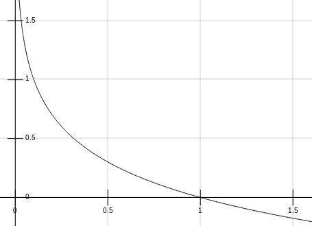
The negative logarithm seems to be a natural choice for this relationship but we can justify the usage of the negative logarithm from a better perspective:

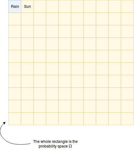
What is the ideal self-information for an event x. For example I(Rain)? Let’s divide the probability space into subspaces of the size of the smallest probability unit. So in our example we could draw a rectangle (which illustrates the probability space omege), divide it into 100 cells of the same size. Each cell shall be part of an event \(x \in \Omega\). The more likely the event is, the more space will it cover. In our example: 99 cells belong to the event Sun and only one cell to the event Rain.

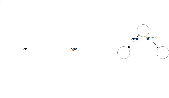
Imagine that we split the probability space recursively at halfs to form a binary tree. The root in this tree divides the space into two areas with probability split 50% to 50%. Stepping down into the left subtree has the code symbol “0” attached and to the right subtree a “1”. The sequence of “0”s and “1”s is what we call the code of the leaf node where we end up. We repeat the splitting until the granularity is fine enough to capture the smallest probability of our events (in our case 1%).

Obviously this depends on the smallest probability. For an Event x with probability P(x) the amount of cells in the probability space is number_cells = 1/P(x). For example for rain P(rain) = 0.01 => number_cells = 1/0.01 = 100

With the splitting from above we can form a binary tree that has 100 leaf nodes (rounding errors are omitted). To answer the question for the optimal encoding for the event “Rain” we only have to find the highest level at which the probability space is divided fine-granular enough to contain a cell with the correct probability.

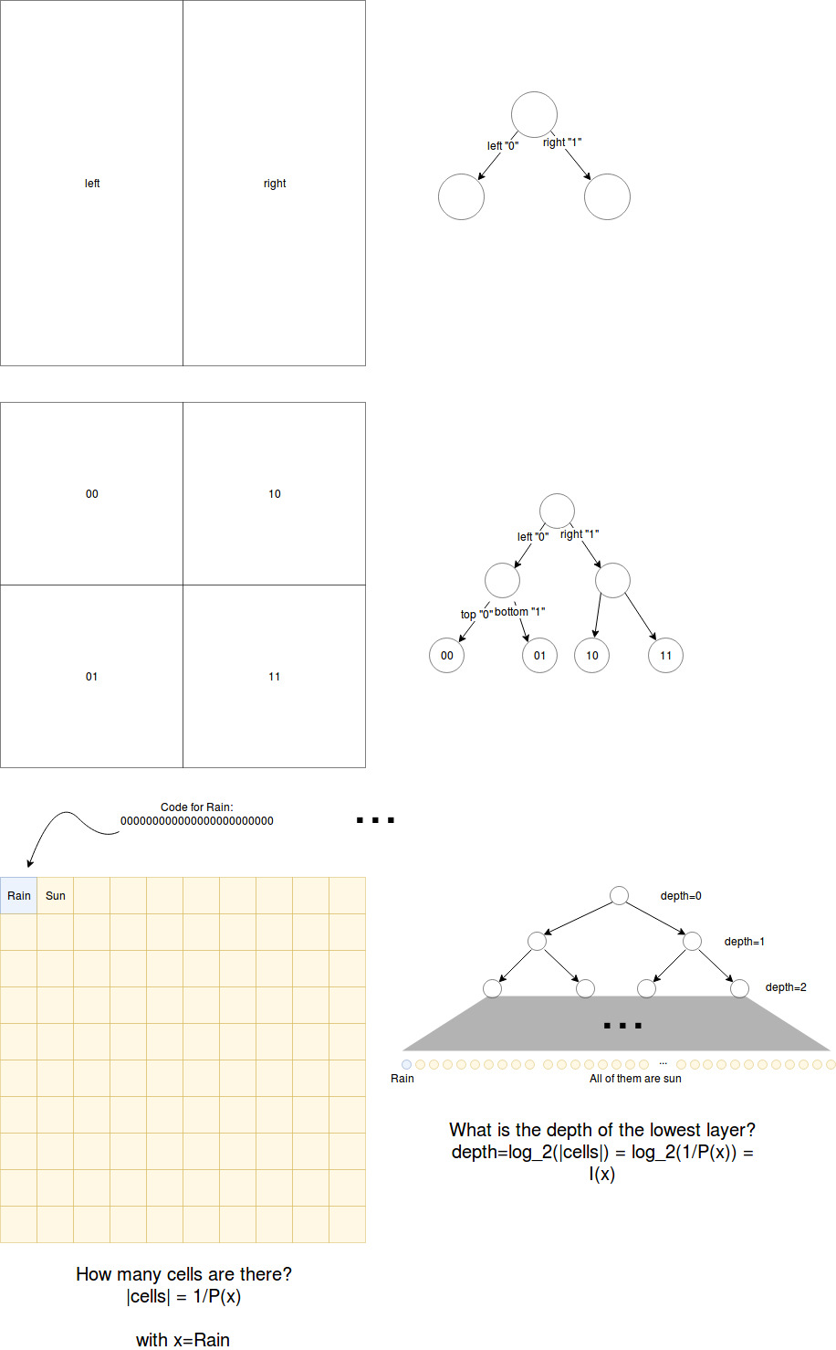
For a binary tree we know that the amount of nodes k at a given depth d is \(k = 2^d\). We start to count the depth at 0. We can transform this to answer the question about the depth: \(d = log_{2}{k}\)

With k=number_cells we get the formula for the self-information I:

\[I(x) = log_{2}{(\frac{1}{P(x)})}\]

This is equivalent to a more typical form: \(I(x) = -log_{2}{(P(x))}\)

Of course we could use a tree with a branching factor different to 2. The base=2 means that our discrete alphabet has two symbols. We know some of these alphabets:

• bits/shannons: base=2
• nats: base=e
• trits: base=3
• dits/hartleys: base=10

Self-information tells us the optimal length to encode the event x.

We can calculate the length of the code for a sequence with this. For example, we might receive the following sequence: “S,S,S,S,S,S,S,S,S,Rain”

We just have to sum over:

• 9 times Sun: 9 times the optimal length for the event sun => 9 * I(Sun)
• 1 times Rain: 1 * I(Rain)

Shannon entropy

But what if we don’t have a given message and we are just interested in the general case aka the mean case. So what would be the message length if we received infinitely many sequences from the channel.

Until now we only calculate the expected self-information of a single event x. For example for Rain or Sun. But we know that these two events are transmitted over the same channel. This is the reason why we might ask ourselves: What is the expected information of the whole channel?

We define the random variable \(X\) from which we draw a sequence of small \(x\). In our example: \(Rain \in X\) and \(Sun \in X\)

We can rephrase the question from above: What is the expected information drawn from an event from X. The expectation value means that we infinitely often draw an event x from X and calculate the mean of the I(x).

Let’s say we draw n samples with \(n \rightarrow \infty\)

\[\mathbb{E}_{x \sim P}[I(x)] = 1/n * \sum_{i=1}^{n}{I(x_i)}\]

We can split the sum into |X| different sums (“distinct events of X”). For every event x one sum. And we know, that every event x should appear P(x) * n times in the sum. For example if drew 100 events from our friend’s weather sequences we “expect” that 100 * 0.01 events of rain should be in there. Which is 1.

\[\begin{equation} \begin{split} \mathbb{E}_{x \sim P}[I(x)] & = 1/n * \sum_{i=1}^{n}{I(x_i)} \\ & = 1/n * \sum_{x_i \in X}{P(x) * n * I(x)} \\ & = 1/n * n * \sum_{x_i \in X}{P(x) * I(x)} \\ & = \sum_{x_i \in X}{P(x) * I(x)} \\ & = H(x) \end{split} \end{equation}\]

That’s it! H(x) is called the Shannon Entropy H(x):

\[H(x) = \mathbb{E}_{x \sim P}[I(x)] = \sum_{x_i \in X}{P(x) * I(x)}\]

Because the probability distribution P is so central to this measure we denote the shannon entropy H(P).

In our example: H(P) = P(Sun) * I(Sun) + P(Rain) * I(Rain) = 0.99 * log_2(1/0.99) + 0.01 * log_2(1/0.01) ~= 0.08

So when your friend calls you the information transmitted is 0.08 bits ;)

We observe that a low entropy means that we know what to expect when we draw an event from a channel. Whereas a low entropy means that there is a high uncertainty.

This is the reason why entropy is called the measure of surprise of a channel.

If P is a uniform distribution for example P(rain) = P(sun) = 0.5 then H(P) is at its maximum which is H(P) = 0.5 * log(1/0.5) + 0.5 * log(1/0.5) = 2 * (0.5 * log(1/0.5)) = 2 * (0.5 * log_2(2)) = 2 * (0.5 * 1) = 2 * 0.5 = 1

Cross entropy

Let’s start with the example again: Imagine that you also have a second friend who lives in the same town as the first friend. The 2nd friend also calls you to also tell you the weather every morning.

Now you are wondering: How many errors happen here? Both sequences should be the same, therefore the probability distributions P and Q should be equal. P is estimated from the sequence of the first friend and Q from the 2nd friend.

We can use the concept of entropy to compare two probability distributions P and Q over the same random variable X. (It has to be the same random variable, don’t get this confused with the conditional entropy which I explain in a later part of this post.)

Main idea: What is the entropy of the sequence of the first friend if we use the probability distribution Q of the 2nd friend to calculate it.

\[\begin{equation} \begin{split} H(P,Q) = \mathbb{E}_{x \sim P}[I_{Q}(x)] & = \mathbb{E}_{x \sim P}[log(1/Q(x))] \\ & = \sum_{x \in X}{P(x) \cdot log(\frac{1}{Q(x)})} \end{split} \end{equation}\]

(formula of cross entropy)

Let’s have a look at three examples to get a feeling for the cross entropy:

• First Example: Let’s say that the 2nd friend reports less rain -> Q(Sun) = 0.999, Q(Rain) = 0.001 Then H(P,Q) = P(Sun) * log(1/Q(Sun)) + P(Rain) * log(1/Q(Rain)) = 0.99 * log_2(1/0.999) + 0.01 * log_2(1/0.001) ~= 0.101
• Second Example: The friends tell you the same things -> P=Q \(H(P,P) = \sum_{x \in X}{P(x) \cdot log(\frac{1}{P(x)})} = H(P)\)
• Third example: the 2nd friend reports more rain -> Q(Sun) = 0.981, Q(Rain) = 0.019 Then H(P,Q) = P(Sun) * log(1/Q(Sun)) + P(Rain) * log(1/Q(Rain)) = 0.99 * log_2(1/0.981) + 0.01 * log_2(1/0.019) ~= 0.085

Observations:

• We observe that the cross entropy is equal to the entropy if P==Q.
• The function is not symmetric
• The higher the distance to the entropy, the more are the distributions divergent

Kullback-Leibler divergence

We have seen that the cross entropy always contains the entropy: \(H(P,Q) = H(P) + divergence_of_P_and_Q\)

This “divergence_of_P_and_Q” is used a lot and has its own name: Kullback-Leibler divergence \(D_{KL}(P \parallel Q)\).

\[H(P,Q) = H(P) + D_{KL}(P \parallel Q)\]

Follows:

\[\begin{equation} \begin{split} D_{KL}(P \parallel Q) &= H(P,Q) - H(P) \\ & = \mathbb{E}_{x \sim P}[I_{Q}(x)] - \mathbb{E}_{x \sim P}[I_{P}(x)] \\ & =\mathbb{E}_{x \sim P}[I_{Q}(x) - I_{P}(x)] = \\ & =\mathbb{E}_{x \sim P}[log (1/Q(x)) - log (1/P(x))] = \\ & =\mathbb{E}_{x \sim P}[log (\frac{1/Q(x)}{1/P(x)})] = \\ & =\mathbb{E}_{x \sim P}[log (\frac{\frac{1}{Q(x)}}{\frac{1}{P(x)}})] = \\ & = \mathbb{E}_{x \sim P}[log \frac{P(x)}{Q(x)}] = \\ & =\mathbb{E}_{x \sim P}[log(P(x)) - log(Q(x))] \end{split} \end{equation}\]

The last term show that when P and Q are equal, the \(D_{KL}(P \parallel Q)\) becomes zero.

Observations:

• From the observation about the cross entropy we can conclude that the KL-divergence is also not symmetrical -> therefore it is per definition not a distance measure => \(D_{KL}(P \parallel Q) \ne D_{KL}(Q \parallel P)\)
• \(D_{KL}(P \parallel Q)\) is always positive
• The Kullback-Leibler divergence has a nice intuition for probability distributions. Namely how many additional bits do we need to encode a message with the true probability distribution P if we are using a coding scheme that was developed using the prob. dist. Q

Log loss

In machine learning we often use something called the “log loss”. For example when we train a neural network for classification. In this case we usually have training data X and a one-hot-encoded label y. The network gets fed the data X. The data is feed forward through the network. As a last layer we often find the softmax function which outputs a vector that sums up to one and every value lies between 0 and 1. This is enough to count as a probability distribution (although we have not checked the sigma-addition).

The output of the network after the softmax is denoted ŷ as it is the estimator for the true label y. To train the neural network we would like to minimize the difference between y and ŷ.

We could just compare the two and say that the error is 1 if they are not the same and 0 if they are. But this would yield a step function which has the disadvantage of having no gradient at important places. That is bad because we need the gradient to perform gradient descent…

Therefore we treat y and ŷ as probability distributions and calculate the cross entropy between them.

\[H(Y, Ŷ) = \sum_{class ~ c}{Y(c) \cdot log( \frac{1}{Ŷ(x)} )}\]

Because for classification there is only one correct class, we know that:

• For all classes which are not the true class c’: \(Y(c)=0\)
• And for the true class c’: \(Y(c') = 1\)

\[\begin{equation} \begin{split} H(Y, Ŷ) &= Y(c^{'}) * log( \frac{1}{Ŷ(c^{'} )}) \\ &= 1 * log( \frac{1}{Ŷ(c^{'} )}) \\ &= log( \frac{1}{Ŷ(c^{'} )}) \\ &= -log(Ŷ(c^{'})) \end{split} \end{equation}\]

The last line is what we call log loss. It can be found everywhere. In tensorflow tf.losses.log_loss or in sckit sklearn.metrics.log_loss…

It has the advantage that we only have to calculate the log of a single value.

Conditional entropy

With the two mentioned friends you can be pretty sure to know the weather in the town. We will call the weather in the town “random variable X”.

Then there is this third friend of you :D She is selling ice cream in the same town. On a daily basis she informs you whether she sold ice cream today (“Ice”) or not (“No ice”). We call this random variable Y.

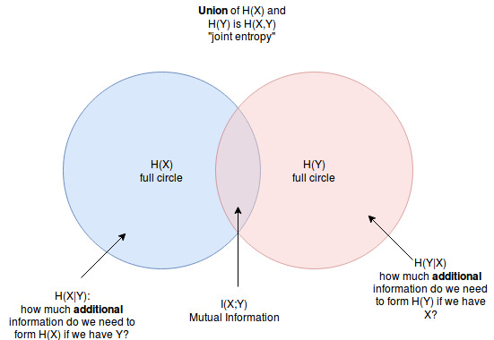
Now you are wondering: How much additional information is necessary to tell whether she sold Ice Cream if we have the weather information (X) from the other two friends?

This can be calculated using the conditional entropy H(Y|X). Speak: Y conditioned on X. Intuitively we can say, if the two events are independent of each others we have to store the entire sequence of Y as if X did not exist. If they are the same we don’t have to store anything additionally.

The formula:

\[\begin{equation} \begin{split} H(Y|X) &= \sum_{x \in X} {( P(x) \cdot \sum_{y \in Y}{P(y|x) \cdot log( \frac{1}{P(y|x)} )} )}\\ &= - \sum_{x \in X} ( P(x) \cdot \sum_{y \in Y}{P(y|x) \cdot log(P(y|x)} ) = \\ &= - \sum_{x \in X} (\sum_{y \in Y}{ P(x) P(y|x) \cdot log(P(y| x)} ) = \\ &= - \sum_{x \in X} (\sum_{y \in Y}{ P(x,y) \cdot log(P(y|x)} ) = \\ &= - \sum_{x \in X, y \in Y} P(x,y) \cdot logP(y|x) = \\ \end{split} \end{equation}\]

(conditional entropy)

observations:

• \(H(Y\vert X) = 0\), if H(Y)=H(X) -> “no additional information”
• \(H(Y\vert X) = H(Y)\), iff X and Y are independent random variables

Joint entropy

We can define a random variable Z which is the union of X and Y. P(Z) = P(X,Y)

According to this we can “extend” the entropy definition to:

\[H(Z) = H(X,Y) = \sum_{x \in X, y \in Y}{P(x,y) \cdot I(x,y)}\]

Mutual Information

The mutual information H(X;Y) is the entropy of the intersection of two random variables X and Y. It captures the dependence of two variables.

\(I(X;Y) = MI(X;Y) = H(X) - H(X|Y)\) (Mutual Infor)

Mutual information maximization estimation (MMIE) can be used to train speech recognition systems.

Perplexity

\(2^{H(P)}\) is called perplexity in speech recognition. It can be interpreted as the average branching factor in language models (for example a context-sensitive grammar). The lower the perplexity the less ambiguities have to be resolved by the acoustic model of the speech recognition system.

Entropy distance

In ASR we got introduced to the entropy distance and the weighted entropy distance. The context was the Kai-Fu Lee Clustering for subtriphones. For every subtriphone you have to train a semi-continuous HMM on the pool of Gaussians. Then we can use the mixture weights of the Gaussians as a probability distribution. Now we can calculate the entropy distance between two subtriphones to get a distance measure. The closest subtriphones are merged together. The big advantage was that we don’t have to train a new HMM for the merged cluster but we can just calculate the weighted sum of the two probability distributions.

The entropy distance: \(d(P, Q) = H(P+Q) - 0.5 H(P) - 0.5 H(Q)\)

The subtriphones differed in the amount of samples in the training data. We want to trust the clusters with fet data points less than the clusters with many data points. This is expressed in the weighted entropy distance:

\[d(P, Q) = (n_{P} + n_{Q})H(P+Q) - n_{P} H(P) - n_{Q} H(Q)\]