Some impressions of LSTM architectures for simple math functions: seq2seq, seq2vec and then seq-seq-autoencoder. In particular the last part is an experiment of reconstructing sinoid waves with phase displacement from a single latent parameter.
Sequence to sequence
X-Y
I generated a line and hill like mapping from points f:X->Y. A one layered LSTM (SGD with fixed learning rate) was able to approx. the line:
In order to get the hill-shaped function I added a second lstm layer (I guess this has the same reason as the XOR “problem”):
In general what this network learned should only be the identity function. It received some coordinates x and y and tried its best to reproduce the same.
Only Y
The following step was to remove the x value from the input so the lstm only received the y-values. It took a little bit longer but the function got approximated:
Sine
The next function I wanted to approximate was a sine:
Which worked out:
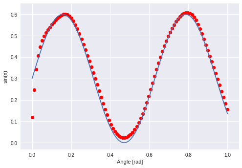
The “learning” of this network should be a little bit more. A temporal dependency between values which was the x-axis in the former example.
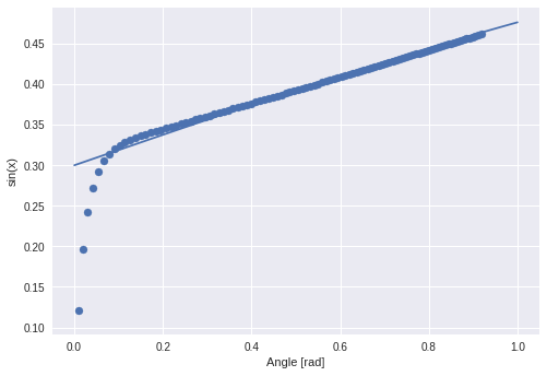
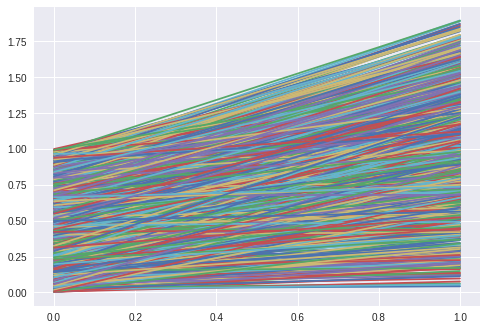
What happens when I feed lines as input to the network?
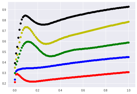
Interestingly they perform something like a sine phase in the beginning and then they grow all by the same factor although their slopes differed from 0.1 to 1.2.
Let’s plot this again without y-intercept.
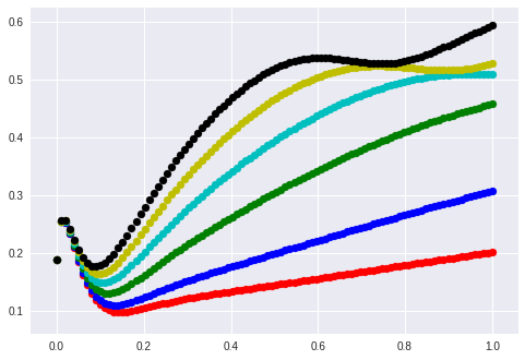
The linear functions are mapped to non-linear functions through the lstm.
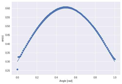
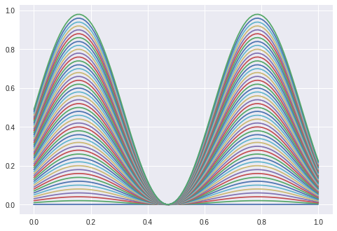
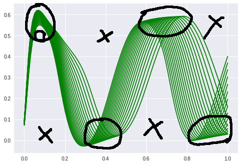
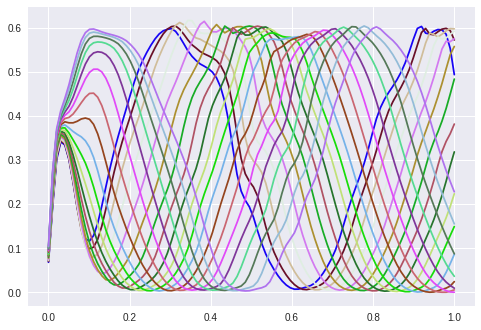
What happens with other sine curves? I start with the same sine with different amplitudes:
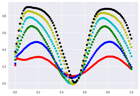
The “learned” sine was in the area between blue and green.
After some graphs I realize that they are actually only interesting if you can see the original function.
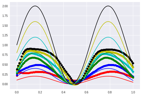
The valley in the middle stays nearly untouched. I guess that this will not be the case when I displace the phase.
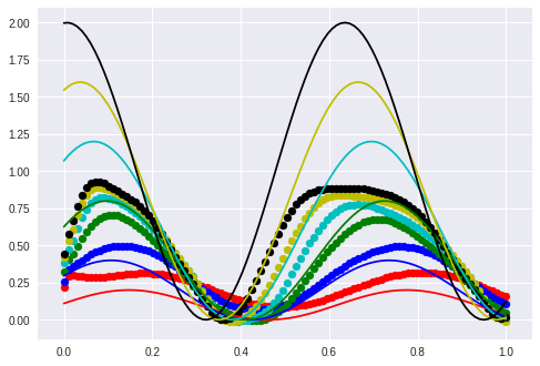
Wrong! The valley stays.
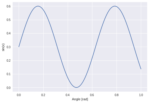
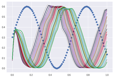
Last chance: Change the frequency…
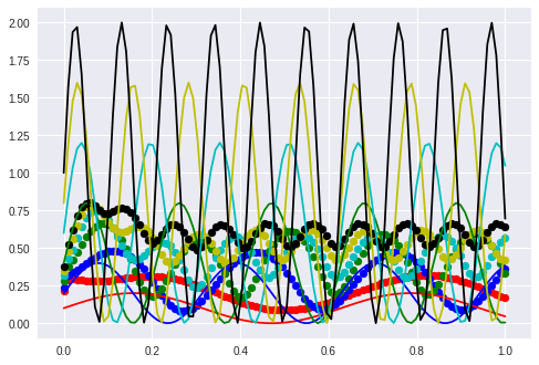
Except for the first part between 0.0 to 0.2 the frequency is copied correctly. It looks as though the only thing that is really wrong is the amplitude.
Sequence to vector
Amplitude of a wave
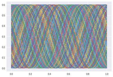
The next task is to extract the amplitude of a sine wave. The lstm gets a sine and is supervised with the sine’s amplitude. The following sines are training examples.
The validation set (from which the following curves are taken) have amplitudes greater than 0.5 (upper bound of ampl. from training set).
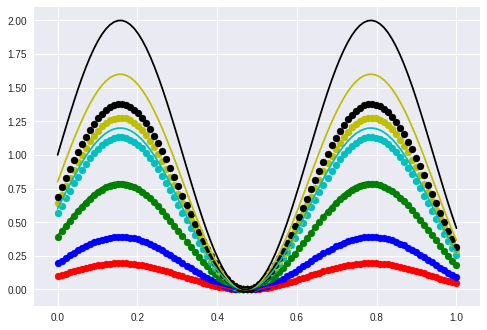
This explains the divergence starting from 0.5 in this plot. Dotted curves are with amplitude from lstm, solid curves groundtruth.
Slope and intercept
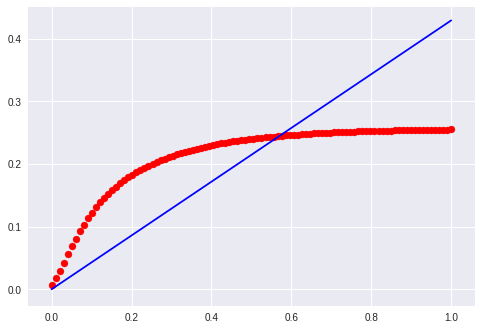
The next task is to learn the slope and intercept of a line.
The hidden function is $f(x) = mx + t$ and the seq2vec lstm is trained to return the parameters (m, t).
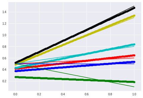
The thin line is the ground truth and the thick line is the “prediction”. Neither negative slope nor a larger slope are handled correctly.
Autoencoder
Sequence to vector and then vector to sequence. Two layered LSTM with a hidden state
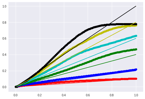
Line
The LSTM creates a hidden representation of a line and shall then regenerate the line from that representation. We know that it should be possible with a vector of 2 entries if it learns “our” linear model.
sizeof(latent) = 10
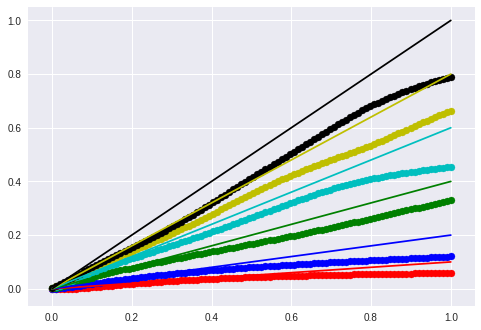
5
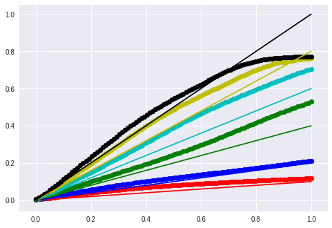
1
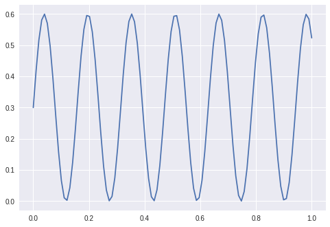
Sine
I just came back from a session with my advisor at university and a third person told us that he was not able to “learn” the sine and cosine function with lstm.
So I generate a sine:
Have the following simple keras code:
from keras.layers import Input, Dense, LSTM, RepeatVector
from keras.models import Model, Sequential
from keras.initializers import RandomNormal, lecun_normal

def get_model(latent_dim=1):

  model = Sequential()
  model.add(LSTM(32, input_shape=(timesteps, input_dim), return_sequences=True))
  model.add(LSTM(latent_dim, return_sequences=False))

  # repeat the latent vector in order to
  # feed it to the next lstm
  model.add(RepeatVector(timesteps))

  model.add(LSTM(32, input_shape=(timesteps, latent_dim), return_sequences=True))
  model.add(LSTM(1, return_sequences=True))

  print(model.summary())

  return model
I train with default MSE and rmsprop:
model = get_model(latent_dim=1)

model.compile(loss='mean_squared_error', optimizer='rmsprop')

for i in range(25):
  model.fit(x_train, x_train,
            epochs=10,
            batch_size=batch_size,
            shuffle=True,
            validation_data=(x_val, x_val))

  training_sample = x_train[np.random.randint(x_train.shape[0])]
  predicted = model.predict(training_sample.reshape(1, timesteps, input_dim))
  plt.scatter(x, predicted, c='r')
  plt.plot(x, training_sample, c='b')

  plt.show()
_________________________________________________________________
Layer (type)                 Output Shape              Param #
=================================================================
lstm_5 (LSTM)                (None, 100, 32)           4352
_________________________________________________________________
lstm_6 (LSTM)                (None, 1)                 136
_________________________________________________________________
repeat_vector_2 (RepeatVecto (None, 100, 1)            0
_________________________________________________________________
lstm_7 (LSTM)                (None, 100, 32)           4352
_________________________________________________________________
lstm_8 (LSTM)                (None, 100, 1)            136
=================================================================
Total params: 8,976
Trainable params: 8,976
Non-trainable params: 0
Sine and cosine
Maybe I understood him wrong. He said something like “I wanted to enter zero and get cosine, and one then get sine”.
There could potentially be a lot of interpretations for this but the output is understandable. He wants to input 0 or 1 and get cosine or sine.
We could do this by inputting arbitrary numbers and expect different outcomes although this seems to be wrong because it is not a sequence. The more I think about it the more it sounds like the problem is framed in the wrong way.
Let’s just do it…
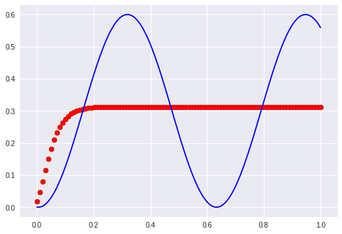
The same lstm gets as input a lot of zeros if we want an cosine and a lot of ones if we want the sine: f(0,0,0,0,0,0,0,..) = cos(x) and f(1,1,1,1,1,1,…) = sin(x)
My assumption is that it learns sinus displaced between the phase of sin and cos. What it did was to learn one perfectly and ignore the other one…
… thinking out loud again: It does not matter too much how he wanted to solve it but that the mapping has to be learned. So I am going to change the architecture to a sequence to sequence autoencoder:
from keras.layers import Input, Dense, LSTM, RepeatVector
from keras.models import Model, Sequential
from keras.initializers import RandomNormal, lecun_normal

def get_model(latent_dim=1):

  inputs = Input(shape=(timesteps, input_dim))
  encoded = LSTM(32, input_shape=(timesteps, input_dim), return_sequences=True)(inputs)
  encoded = LSTM(32, input_shape=(timesteps, input_dim), return_sequences=True)(encoded)
  encoded = LSTM(latent_dim, input_shape=(timesteps, input_dim), return_sequences=False)(encoded)

  latent_state = RepeatVector(timesteps)(encoded)

  decoded = LSTM(32, input_shape=(timesteps, input_dim), return_sequences=True)(latent_state)
  decoded = LSTM(32, input_shape=(timesteps, input_dim), return_sequences=True)(decoded)
  decoded = LSTM(1, input_shape=(timesteps, input_dim), return_sequences=True)(decoded)

  autoencoder = Model(inputs, decoded)

  # decoder
  encoded_input = Input(shape=(latent_dim,))
  deco = autoencoder.layers[-4](encoded_input)
  deco = autoencoder.layers[-3](deco)
  deco = autoencoder.layers[-2](deco)
  deco = autoencoder.layers[-1](deco)

  # create the decoder model
  decoder = Model(encoded_input, deco)

  # encoder
  encoder = Model(inputs, encoded)

  print(autoencoder.summary())

  return autoencoder, decoder, encoder
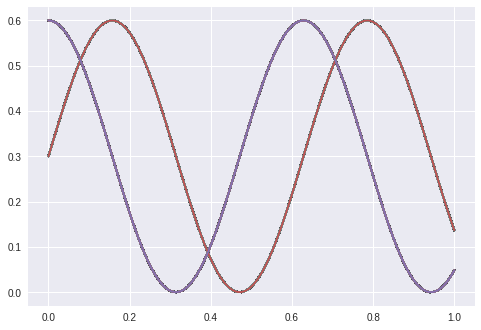
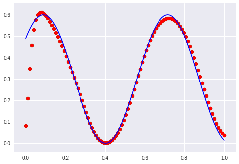
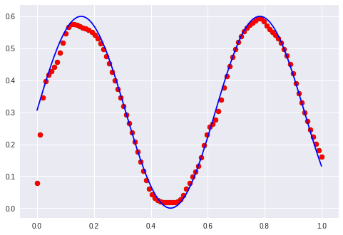
I feed it a sine with a given phase displacement and it shall reconstruct the sine with one latent parameter.
Which works:
Now I interpolate in the linear space of the latent variable from -1 to -0.5 and the following image shows what I get:
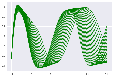
So by changing the latent value we can displace the phase of the sine (except for the beginning, which also has problems reconstructing but it gets better slowly when trained more epochs).
Now the phase displacement was just 0.1 * pi/2. To scale this solution up to the “task” I have to increase the maximum displacement to pi/2 which is the shift of sine to cosine: sin(x+pi/2) = cos(x).
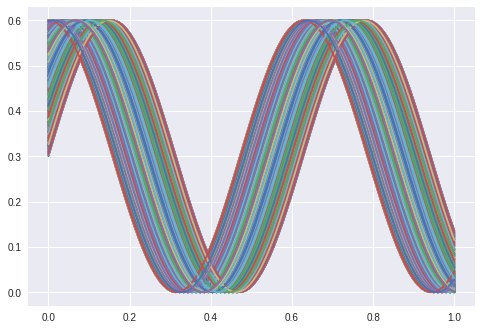
That this is a much harder problem is obvious when we look at the training data:
The first examples with waves “formed” the manifold just to route the sines over a given point. This is not possible anymore. It is interesting to note that the network needs a far longer time to start bending the predicted curve. It stayes parallel to the x-axis for at least 100 epochs.
After 150 epochs the sine waves start to become reconstructed:
100 epochs later the cosine gets approximated:
I have to mention that this training was done with Adam and not with rmsprop anymore.
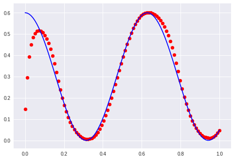
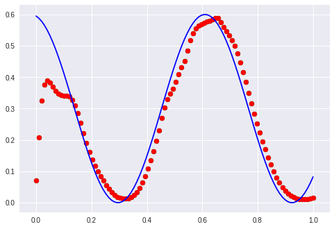
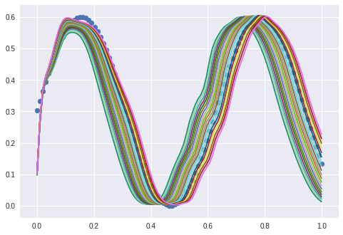
Result: Interpolating the hidden value between 0.5 and 1.0 results in phase displaced waves:
I still have the problem in the area of x < 0.2, but the rest looks good.
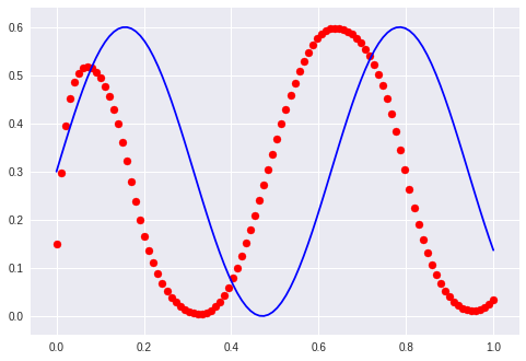
If I only interpolate between 0.6 to 0.8 I get good enough cosine waves. (Blue points is the sine for reference):
And I can flip this by shifting the interpolation frame to 0.9-1.0:
To conclude this experiment: I can understand how to end up in a dead end street if the architecture is not chosen apropriately. But if the autoencoder is trained in a real “autoencoding” way then the one latent variable can be used directly to control the phase displacement of such a sine wave.
Code autoencoder
Some code snippets for data generation, training and evaluation.
Data generation
# Build an LSTM seq2seq autoencoder
import numpy as np
import matplotlib.pylab as plt
batch_size = 1000
# discretization points N
timesteps = 100
# we only input one point for every timestep
input_dim = 1
# get discrete points between -1 and +1
x = np.linspace(0, 1, timesteps)
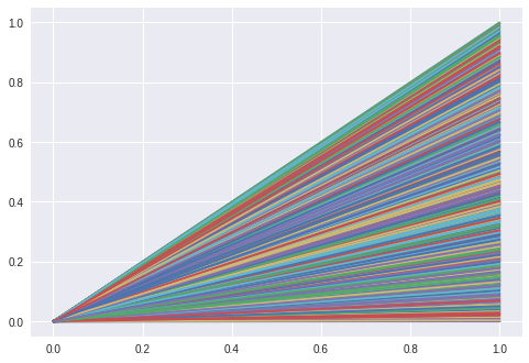
# Training data
x_train = []
y_train = []
for ampl in range(batch_size):
ampl = np.random.random()
intercept = 0
y = ampl * x + intercept
x_train.append(y)
y_train.append([ampl, intercept])
plt.plot(x, y)
x_train = np.array(x_train).reshape(-1, timesteps, input_dim)
y_train = np.array(y_train).reshape(-1, 2)
# Test data (DRY :D)
x_val = []
y_val = []
for ampl in range(batch_size//10):
ampl = np.random.random()
intercept = 0
y = ampl * x + intercept
x_val.append(y)
y_val.append([ampl, intercept])
x_val = np.array(x_val).reshape(-1, timesteps, input_dim)
y_val = np.array(y_val).reshape(-1, 2)
plt.axis('tight')
plt.show()
Build the model
from keras.layers import Input, Dense, LSTM, RepeatVector
from keras.models import Model, Sequential

def get_model(latent_dim=5):

  model = Sequential()
  model.add(LSTM(32, input_shape=(timesteps, input_dim), return_sequences=True))
  model.add(LSTM(latent_dim, return_sequences=False))

  # repeat the latent vector in order to
  # feed it to the next lstm
  model.add(RepeatVector(timesteps))

  model.add(LSTM(32, input_shape=(timesteps, latent_dim), return_sequences=True))
  model.add(LSTM(1, return_sequences=True))

  print(model.summary())

  return model
### Training
I used Keras for that and fiddled with different optimizers and parameters. In the end I stayed with RMSprop.
model = get_model(latent_dim=5)

model.compile(loss='mean_squared_error', optimizer='rmsprop')

for i in range(25):
  model.fit(x_train, x_train,
            epochs=10,
            batch_size=batch_size,
            shuffle=True,
            validation_data=(x_val, x_val))

  training_sample = x_train[np.random.randint(x_train.shape[0])]
  predicted = model.predict(training_sample.reshape(1, timesteps, input_dim))
  plt.scatter(x, predicted, c='r')
  plt.plot(x, training_sample, c='b')

  plt.show()
Evaluate
for m, t, color in [
	(0.1, 0.0, 'r'),
    (0.2, 0.0, 'b'),
    (0.4, 0.0, 'g'),
    (0.6, 0.0, 'c'),
    (0.8, 0.0, 'y'),
    (1.0, 0.0, 'k')]:
  lin_x = m * x + t

  seq = model.predict(lin_x.reshape(1,timesteps, input_dim))
  new_y = seq.reshape(-1, input_dim)

  plt.scatter(x, new_y, c=color)
  plt.plot(x, lin_x, c=color)

plt.show()